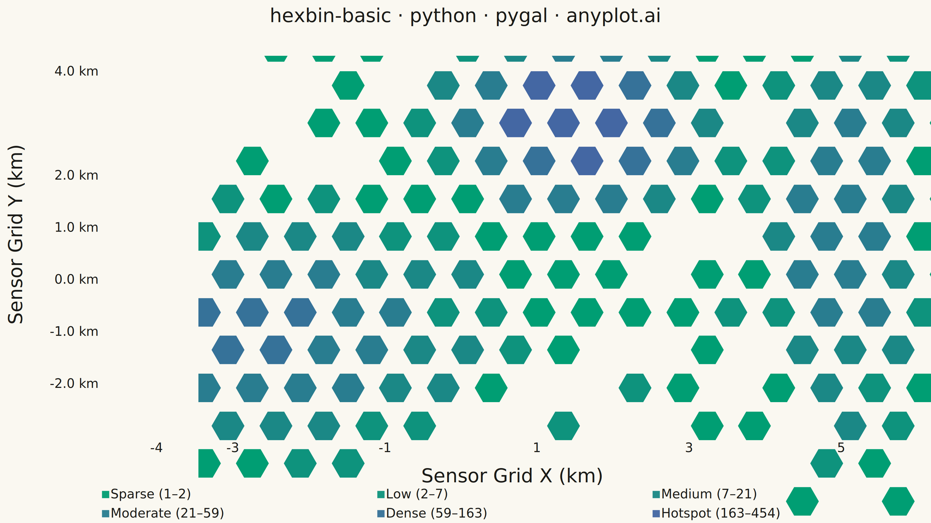
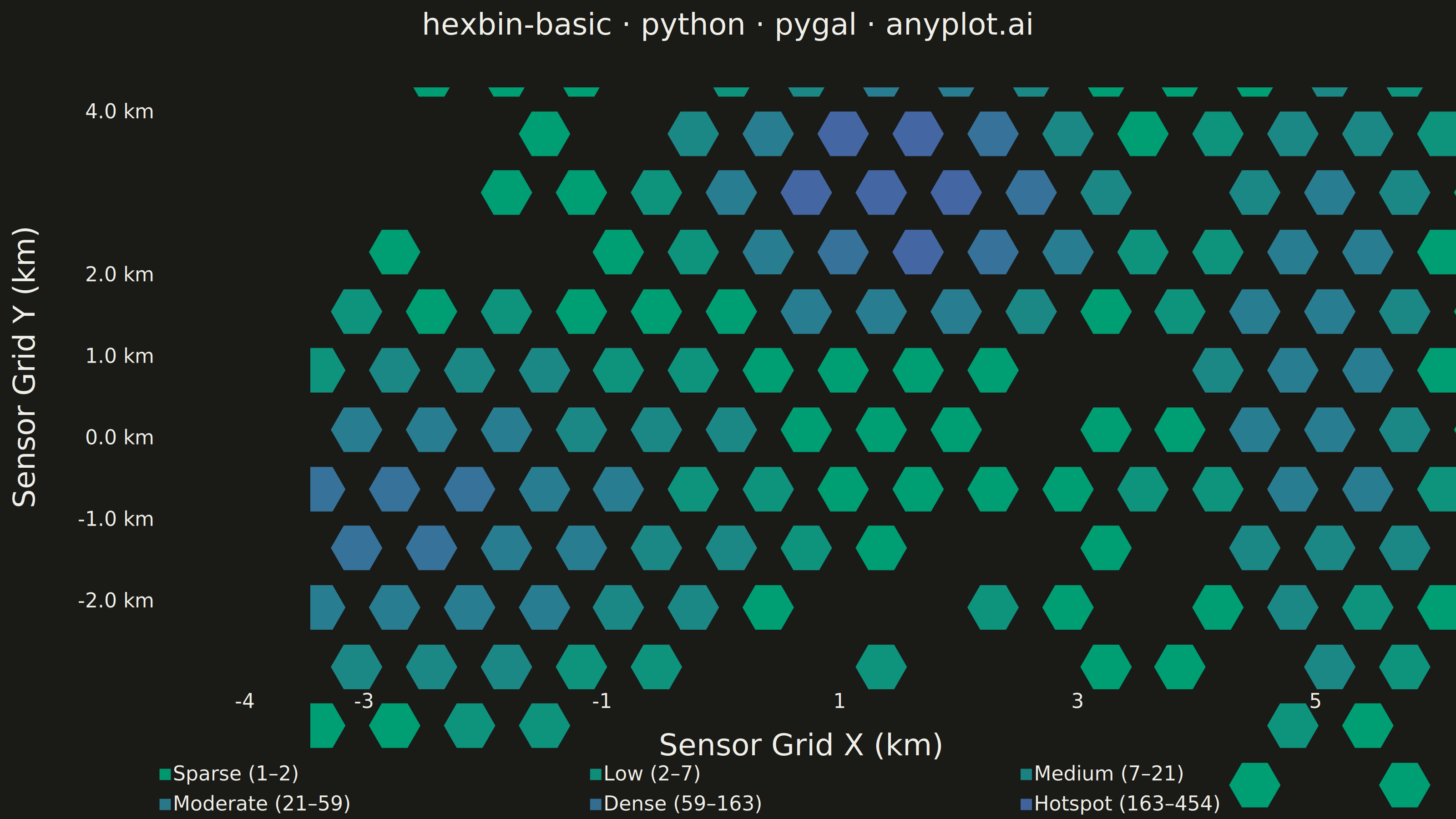
A hexagonal binning plot that visualizes the density of 2D point data by aggregating points into hexagonal bins. The color intensity of each hexagon represents the count of points within it, making it ideal for revealing density patterns in large datasets where traditional scatter plots would show overlapping points. Hexagonal bins provide better visual representation than square pixels due to their isotropy (equal distance to neighboring cells in all directions).
""" anyplot.ai
hexbin-basic: Basic Hexbin Plot
Library: pygal 3.1.0 | Python 3.13.13
Quality: 85/100 | Created: 2026-05-29
"""

import importlib.util
import math
import os
import re
import sys

import cairosvg
import numpy as np


# Ensure we import the installed pygal package, not this file
pygal_spec = importlib.util.find_spec("pygal")
if pygal_spec and pygal_spec.origin != __file__:
    import pygal
    from pygal.style import Style
else:
    cwd = os.getcwd()
    sys.path = [p for p in sys.path if os.path.abspath(p) != cwd]
    try:
        import pygal
        from pygal.style import Style
    finally:
        sys.path.insert(0, cwd)

THEME = os.getenv("ANYPLOT_THEME", "light")

# Theme-adaptive chrome tokens (Imprint style guide)
PAGE_BG = "#FAF8F1" if THEME == "light" else "#1A1A17"
INK = "#1A1A17" if THEME == "light" else "#F0EFE8"
INK_MUTED = "#6B6A63" if THEME == "light" else "#A8A79F"


# Imprint sequential colormap: brand green (#009E73) → blue (#4467A3), sparse → dense
N_LEVELS = 6
density_colors = tuple(
    f"#{round(0x00 + (0x44 - 0x00) * i / (N_LEVELS - 1)):02X}"
    f"{round(0x9E + (0x67 - 0x9E) * i / (N_LEVELS - 1)):02X}"
    f"{round(0x73 + (0xA3 - 0x73) * i / (N_LEVELS - 1)):02X}"
    for i in range(N_LEVELS)
)

# Data: urban air quality sensor network with three pollution hotspots
np.random.seed(42)
core_x = np.random.randn(2500) * 0.6 + 1.5
core_y = np.random.randn(2500) * 0.6 + 3.0
industrial_x = np.random.randn(1200) * 1.1 - 2.5
industrial_y = np.random.randn(1200) * 0.9 - 1.0
highway_x = np.random.randn(600) * 0.4 + 5.0
highway_y = np.random.randn(600) * 1.8 + 1.0
bg_x = np.random.uniform(-4.0, 6.5, 150)
bg_y = np.random.uniform(-3.0, 5.5, 150)

sensor_x = np.concatenate([core_x, industrial_x, highway_x, bg_x])
sensor_y = np.concatenate([core_y, industrial_y, highway_y, bg_y])

# Hexagonal binning: assign points to tessellating hex cells, count per cell
GRIDSIZE = 20
PAD = 0.2
x_min, x_max = sensor_x.min() - PAD, sensor_x.max() + PAD
y_min = sensor_y.min() - PAD

hex_width = (x_max - x_min) / GRIDSIZE  # pointy-top: x-spacing = sqrt(3)*R
hex_height = hex_width * 2 / np.sqrt(3)  # y-spacing = 2R, circumradius R = hex_width/sqrt(3)

rows = ((sensor_y - y_min) / hex_height).astype(int)
odd_shift = np.where(rows % 2 == 1, 0.5, 0.0)
cols = ((sensor_x - x_min) / hex_width - odd_shift).astype(int)

cell_ids = cols * 10000 + rows
unique_cells, counts = np.unique(cell_ids, return_counts=True)
cell_cols = unique_cells // 10000
cell_rows = unique_cells % 10000
cx = x_min + (cell_cols + np.where(cell_rows % 2 == 1, 0.5, 0.0)) * hex_width + hex_width / 2
cy = y_min + cell_rows * hex_height + hex_height / 2

# Log-spaced density thresholds → 6 colour levels
c_min, c_max = float(counts.min()), float(counts.max())
edges = np.logspace(np.log10(c_min), np.log10(c_max + 1), N_LEVELS + 1)
edges[0] = c_min
edges[-1] = c_max + 1

level_names = ["Sparse", "Low", "Medium", "Moderate", "Dense", "Hotspot"]
labels = [f"{level_names[i]} ({int(edges[i])}–{int(edges[i + 1])})" for i in range(N_LEVELS)]

series_data: list[list] = [[] for _ in range(N_LEVELS)]
for x, y, cnt in zip(cx, cy, counts, strict=True):
    level = min(int(np.searchsorted(edges[1:], cnt)), N_LEVELS - 1)
    series_data[level].append({"value": (round(float(x), 2), round(float(y), 2)), "label": f"{int(cnt)} readings"})

# Imprint sequential palette, theme-adaptive chrome
custom_style = Style(
    background=PAGE_BG,
    plot_background=PAGE_BG,
    foreground=INK,
    foreground_strong=INK,
    foreground_subtle=INK_MUTED,
    colors=density_colors,
    opacity=0.95,
    opacity_hover=1.0,
    title_font_size=66,
    label_font_size=56,
    major_label_font_size=44,
    legend_font_size=44,
    value_font_size=36,
    title_font_family="sans-serif",
    label_font_family="sans-serif",
    major_label_font_family="sans-serif",
    legend_font_family="sans-serif",
)

# Axis viewport: 2nd/98th percentile + padding to trim outlier tails
x_lo = float(np.percentile(sensor_x, 2)) - 0.4
x_hi = float(np.percentile(sensor_x, 98)) + 0.4
y_lo = float(np.percentile(sensor_y, 2)) - 0.4
y_hi = float(np.percentile(sensor_y, 98)) + 0.4

# Uniform circumradius for tessellating hexagons (SVG user units = pixels at 3200px width)
# Estimate: plot area ≈ 2900px wide, x_range ≈ 10.8 km, gridsize=20 →
# hex_width_px = 2900/20 = 145, circumradius = 145/sqrt(3) ≈ 84
# Use 56 for crisp gaps between hexes (standard hexbin look) and title headroom
HEX_R = 56

chart = pygal.XY(
    width=3200,
    height=1800,
    style=custom_style,
    title="hexbin-basic · python · pygal · anyplot.ai",
    x_title="Sensor Grid X (km)",
    y_title="Sensor Grid Y (km)",
    show_legend=True,
    legend_at_bottom=True,
    legend_at_bottom_columns=3,
    legend_box_size=24,
    stroke=False,
    dots_size=HEX_R,
    show_x_guides=False,
    show_y_guides=False,
    xrange=(x_lo, x_hi),
    range=(y_lo, y_hi),
    truncate_legend=-1,
    print_values=False,
    human_readable=True,
    x_labels_major_count=6,
    y_labels_major_count=6,
    show_minor_x_labels=False,
    show_minor_y_labels=False,
    value_formatter=lambda v: f"{v:.1f} km",
)

for i in range(N_LEVELS):
    if series_data[i]:
        chart.add(labels[i], series_data[i], dots_size=HEX_R)

# SVG post-processing: replace circle markers with hexagonal polygons
svg_raw = chart.render()
svg_text = svg_raw.decode("utf-8") if isinstance(svg_raw, bytes) else svg_raw


def _circle_to_hex(match: re.Match) -> str:
    tag = match.group(0)
    cx_m = re.search(r'cx="([\d.e+-]+)"', tag)
    cy_m = re.search(r'cy="([\d.e+-]+)"', tag)
    r_m = re.search(r"\br=\"([\d.e+-]+)\"", tag)
    if not (cx_m and cy_m and r_m):
        return tag
    r_v = float(r_m.group(1))
    if r_v < 1.0:  # skip tiny decorative circles (legend dots, etc.)
        return tag
    xc, yc = float(cx_m.group(1)), float(cy_m.group(1))
    pts = " ".join(
        f"{xc + r_v * math.cos(math.radians(a)):.2f},{yc + r_v * math.sin(math.radians(a)):.2f}"
        for a in range(0, 360, 60)
    )
    result = re.sub(r'\bcx="[\d.e+-]+"', "", tag)
    result = re.sub(r'\bcy="[\d.e+-]+"', "", result)
    result = re.sub(r"\br=\"[\d.e+-]+\"", f'points="{pts}"', result, count=1)
    return result.replace("<circle", "<polygon")


svg_hex = re.sub(r"<circle[^>]*/>", _circle_to_hex, svg_text)

# Inject a clip-path for the data area so hexagons don't bleed into title/margins.
# Extract the plot group transform to find the data area bounds in SVG coordinates.
plot_transform_m = re.search(r'<g transform="translate\(([\d.]+),\s*([\d.]+)\)" class="plot"', svg_hex)
plot_bg_m = re.search(r'<rect x="0" y="0" width="([\d.]+)" height="([\d.]+)" class="background"', svg_hex)
if plot_transform_m and plot_bg_m:
    px = float(plot_transform_m.group(1))
    py = float(plot_transform_m.group(2))
    pw = float(plot_bg_m.group(1))
    ph = float(plot_bg_m.group(2))
    clip_id = "hex-data-clip"
    clip_def = (
        f'<clipPath id="{clip_id}"><rect x="{px:.1f}" y="{py:.1f}" width="{pw:.1f}" height="{ph:.1f}"/></clipPath>'
    )
    # Insert clipPath into <defs>
    svg_hex = svg_hex.replace("</defs>", clip_def + "</defs>", 1)
    # Apply clip to each series <g> group (leaves axis/label groups unclipped)
    svg_hex = re.sub(
        r'(<g class="series [^"]*">)', lambda m: m.group(0).replace(">", f' clip-path="url(#{clip_id})">', 1), svg_hex
    )
    # Subtle plot frame — inner background rect from plot group (width/height relative to transform)
    inner_m = re.search(r'<rect[^>]+class="plot_background"[^>]*/>', svg_hex) or re.search(
        r'<rect[^>]+class="graph"[^>]*/>', svg_hex
    )
    if inner_m:
        inner_tag = inner_m.group(0)
        iw_m = re.search(r'width="([\d.]+)"', inner_tag)
        ih_m = re.search(r'height="([\d.]+)"', inner_tag)
        if iw_m and ih_m:
            iw, ih = float(iw_m.group(1)), float(ih_m.group(1))
            frame_svg = (
                f'<rect x="{px:.1f}" y="{py:.1f}" width="{iw:.1f}" height="{ih:.1f}" '
                f'fill="none" stroke="{INK_MUTED}" stroke-width="1.5" opacity="0.3"/>'
            )
            svg_hex = svg_hex.replace("</svg>", frame_svg + "\n</svg>")

# Save interactive HTML and static PNG
with open(f"plot-{THEME}.html", "w", encoding="utf-8") as f:
    f.write(svg_hex)

cairosvg.svg2png(bytestring=svg_hex.encode("utf-8"), write_to=f"plot-{THEME}.png")
Runnable source as JSON, for any HTTP client: https://api.anyplot.ai/specs/hexbin-basic/pygal/code. Any spec id and library id listed in llms-full.txt fit the same URL shape; every URL below is complete and callable.
{
  "spec_id": "hexbin-basic",
  "language": "python",
  "library": "pygal",
  "page": "https://anyplot.ai/hexbin-basic/python/pygal",
  "hub": "https://anyplot.ai/hexbin-basic",
  "code_json": "https://api.anyplot.ai/specs/hexbin-basic/pygal/code",
  "spec_json": "https://api.anyplot.ai/specs/hexbin-basic",
  "render_light_png": "https://storage.googleapis.com/anyplot-images/plots/hexbin-basic/python/pygal/plot-light.png",
  "render_dark_png": "https://storage.googleapis.com/anyplot-images/plots/hexbin-basic/python/pygal/plot-dark.png",
  "interactive_light_html": "https://storage.googleapis.com/anyplot-images/plots/hexbin-basic/python/pygal/plot-light.html",
  "interactive_dark_html": "https://storage.googleapis.com/anyplot-images/plots/hexbin-basic/python/pygal/plot-dark.html",
  "quality_score": 85.0,
  "license": "MIT",
  "guide": "https://anyplot.ai/llms.txt"
}
Part of Basic Hexbin Plot on anyplot.ai.