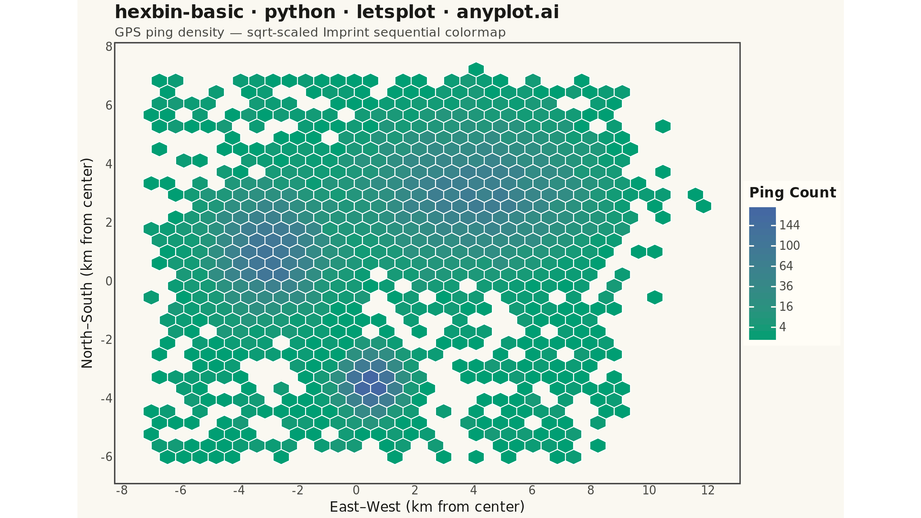
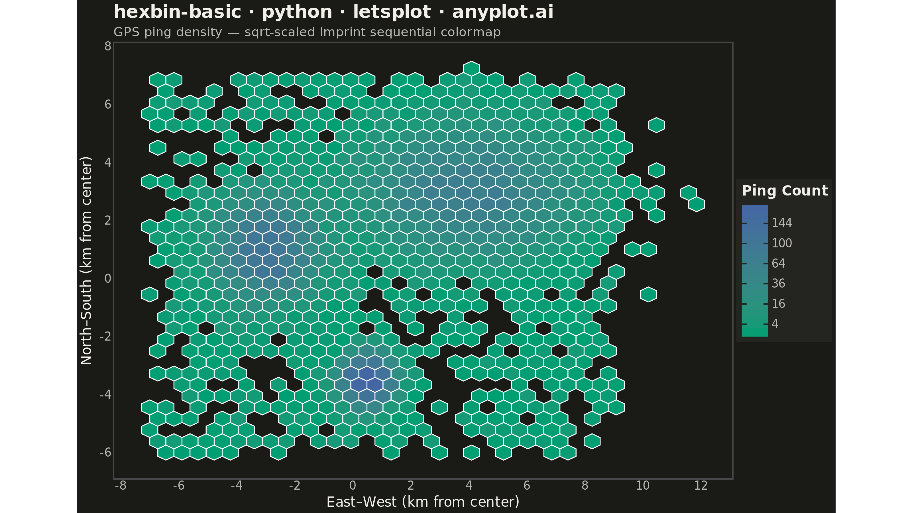
A hexagonal binning plot that visualizes the density of 2D point data by aggregating points into hexagonal bins. The color intensity of each hexagon represents the count of points within it, making it ideal for revealing density patterns in large datasets where traditional scatter plots would show overlapping points. Hexagonal bins provide better visual representation than square pixels due to their isotropy (equal distance to neighboring cells in all directions).
""" anyplot.ai
hexbin-basic: Basic Hexbin Plot
Library: letsplot 4.10.1 | Python 3.13.13
Quality: 92/100 | Updated: 2026-05-29
"""

import os

import numpy as np
import pandas as pd
from lets_plot import (
    LetsPlot,
    aes,
    coord_fixed,
    element_blank,
    element_line,
    element_rect,
    element_text,
    geom_hex,
    ggplot,
    ggsize,
    labs,
    layer_tooltips,
    scale_fill_gradient,
    theme,
    theme_minimal,
)
from lets_plot.export import ggsave


LetsPlot.setup_html()

# Theme tokens (Imprint palette — theme-adaptive chrome)
THEME = os.getenv("ANYPLOT_THEME", "light")
PAGE_BG = "#FAF8F1" if THEME == "light" else "#1A1A17"
ELEVATED_BG = "#FFFDF6" if THEME == "light" else "#242420"
INK = "#1A1A17" if THEME == "light" else "#F0EFE8"
INK_SOFT = "#4A4A44" if THEME == "light" else "#B8B7B0"

# Data - Simulated GPS ping density across a metro area (km from city center)
np.random.seed(42)
n_points = 10000

# Downtown core - elongated east-west along commercial corridor
downtown_east = np.random.randn(n_points // 2) * 2.0 + 4
downtown_north = np.random.randn(n_points // 2) * 1.2 + 3

# University campus - compact circular footprint
campus_east = np.random.randn(n_points // 3) * 1.0 - 3
campus_north = np.random.randn(n_points // 3) * 1.0 + 1

# Transit hub - tight cluster of commuters
transit_east = np.random.randn(n_points // 6) * 0.5 + 0.5
transit_north = np.random.randn(n_points // 6) * 0.5 - 3.5

# Sparse residential pings across outer metro area
bg_east = np.random.uniform(-7, 9, n_points // 10)
bg_north = np.random.uniform(-6, 7, n_points // 10)

east_km = np.concatenate([downtown_east, campus_east, transit_east, bg_east])
north_km = np.concatenate([downtown_north, campus_north, transit_north, bg_north])

df = pd.DataFrame({"east_km": east_km, "north_km": north_km})

# Plot - Hexagonal binning to reveal pedestrian density hotspots
plot = (
    ggplot(df, aes(x="east_km", y="north_km"))
    + geom_hex(
        aes(fill="..count.."),
        bins=[35, 35],
        color="#FFFFFF",
        size=0.3,
        tooltips=layer_tooltips()
        .title("Hex Bin")
        .line("pings|@..count..")
        .line("density|@..density..")
        .format("@..density..", ".3f"),
    )
    + scale_fill_gradient(low="#009E73", high="#4467A3", name="Ping Count", trans="sqrt")
    + coord_fixed()
    + labs(
        x="East–West (km from center)",
        y="North–South (km from center)",
        title="hexbin-basic · python · letsplot · anyplot.ai",
        subtitle="GPS ping density — sqrt-scaled Imprint sequential colormap",
    )
    + theme_minimal()
    + theme(
        plot_background=element_rect(fill=PAGE_BG, color=PAGE_BG),
        panel_background=element_rect(fill=PAGE_BG),
        panel_grid_major=element_blank(),
        panel_grid_minor=element_blank(),
        axis_title=element_text(size=12, color=INK),
        axis_text=element_text(size=10, color=INK_SOFT),
        axis_line=element_line(color=INK_SOFT),
        plot_title=element_text(size=16, face="bold", color=INK),
        plot_subtitle=element_text(size=11, color=INK_SOFT),
        legend_background=element_rect(fill=ELEVATED_BG, color=INK_SOFT),
        legend_text=element_text(size=10, color=INK_SOFT),
        legend_title=element_text(size=12, face="bold", color=INK),
    )
    + ggsize(800, 450)
)

# Save PNG (scale=4 gives 3200×1800)
ggsave(plot, f"plot-{THEME}.png", path=".", scale=4)

# Save HTML for interactive tooltips
ggsave(plot, f"plot-{THEME}.html", path=".")
Runnable source as JSON, for any HTTP client: https://api.anyplot.ai/specs/hexbin-basic/letsplot/code. Any spec id and library id listed in llms-full.txt fit the same URL shape; every URL below is complete and callable.
{
  "spec_id": "hexbin-basic",
  "language": "python",
  "library": "letsplot",
  "page": "https://anyplot.ai/hexbin-basic/python/letsplot",
  "hub": "https://anyplot.ai/hexbin-basic",
  "code_json": "https://api.anyplot.ai/specs/hexbin-basic/letsplot/code",
  "spec_json": "https://api.anyplot.ai/specs/hexbin-basic",
  "render_light_png": "https://storage.googleapis.com/anyplot-images/plots/hexbin-basic/python/letsplot/plot-light.png",
  "render_dark_png": "https://storage.googleapis.com/anyplot-images/plots/hexbin-basic/python/letsplot/plot-dark.png",
  "interactive_light_html": "https://storage.googleapis.com/anyplot-images/plots/hexbin-basic/python/letsplot/plot-light.html",
  "interactive_dark_html": "https://storage.googleapis.com/anyplot-images/plots/hexbin-basic/python/letsplot/plot-dark.html",
  "quality_score": 92.0,
  "license": "MIT",
  "guide": "https://anyplot.ai/llms.txt"
}
Part of Basic Hexbin Plot on anyplot.ai.