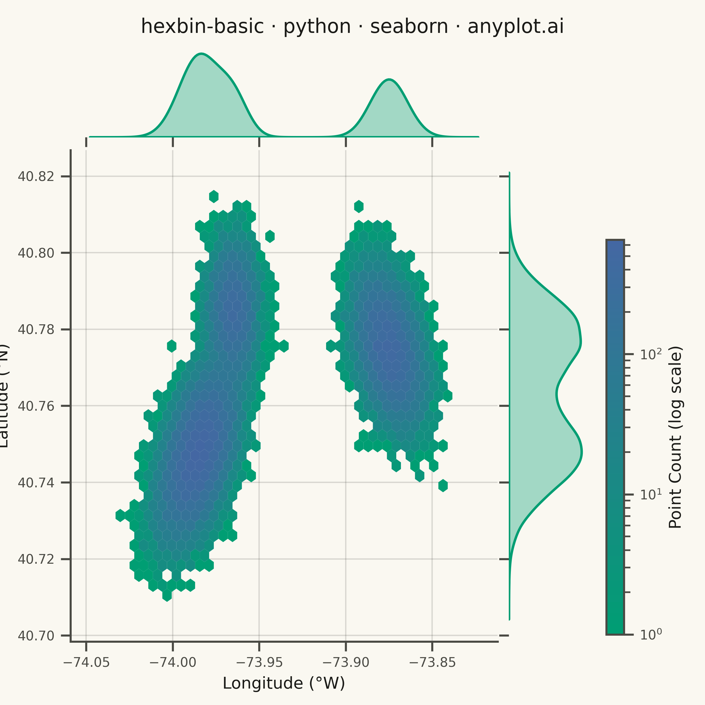
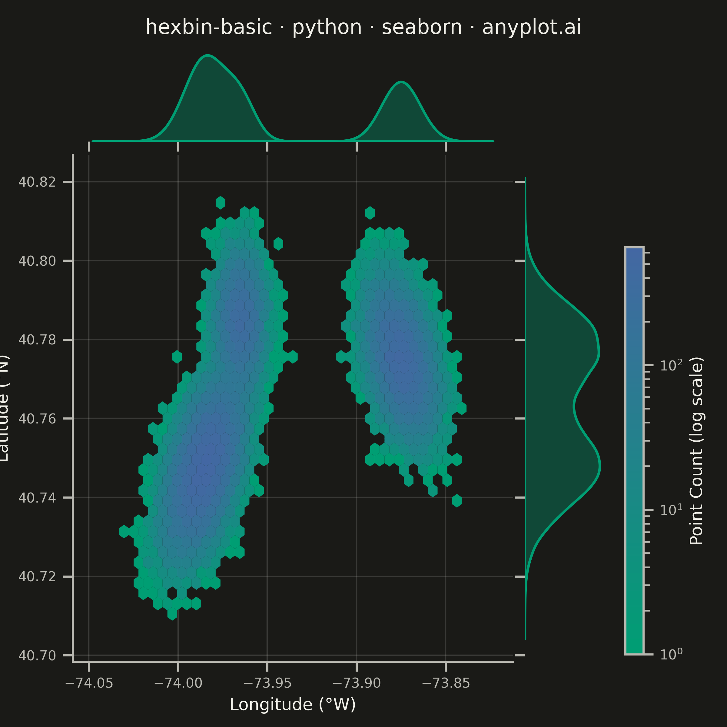
A hexagonal binning plot that visualizes the density of 2D point data by aggregating points into hexagonal bins. The color intensity of each hexagon represents the count of points within it, making it ideal for revealing density patterns in large datasets where traditional scatter plots would show overlapping points. Hexagonal bins provide better visual representation than square pixels due to their isotropy (equal distance to neighboring cells in all directions).
""" anyplot.ai
hexbin-basic: Basic Hexbin Plot
Library: seaborn 0.13.2 | Python 3.13.13
Quality: 91/100 | Updated: 2026-05-29
"""

import os

import numpy as np
import seaborn as sns
from matplotlib.colors import LinearSegmentedColormap, LogNorm


# Theme tokens
THEME = os.getenv("ANYPLOT_THEME", "light")
PAGE_BG = "#FAF8F1" if THEME == "light" else "#1A1A17"
ELEVATED_BG = "#FFFDF6" if THEME == "light" else "#242420"
INK = "#1A1A17" if THEME == "light" else "#F0EFE8"
INK_SOFT = "#4A4A44" if THEME == "light" else "#B8B7B0"

# Imprint sequential colormap for continuous density data
imprint_seq = LinearSegmentedColormap.from_list("imprint_seq", ["#009E73", "#4467A3"])

# Data — NYC GPS coordinates for urban traffic hotspot analysis
np.random.seed(42)
n_points = 50000

downtown = np.random.multivariate_normal([-73.985, 40.748], [[0.0001, 0.00005], [0.00005, 0.0001]], n_points // 2)
airport = np.random.multivariate_normal([-73.875, 40.775], [[0.00008, -0.00003], [-0.00003, 0.00008]], n_points // 3)
shopping = np.random.multivariate_normal([-73.965, 40.785], [[0.00004, 0], [0, 0.00006]], n_points // 6)

longitude = np.concatenate([downtown[:, 0], airport[:, 0], shopping[:, 0]])
latitude = np.concatenate([downtown[:, 1], airport[:, 1], shopping[:, 1]])

# Plot
sns.set_theme(
    style="ticks",
    rc={
        "figure.facecolor": PAGE_BG,
        "axes.facecolor": PAGE_BG,
        "axes.edgecolor": INK_SOFT,
        "axes.labelcolor": INK,
        "text.color": INK,
        "xtick.color": INK_SOFT,
        "ytick.color": INK_SOFT,
        "grid.color": INK,
        "grid.alpha": 0.15,
        "legend.facecolor": ELEVATED_BG,
        "legend.edgecolor": INK_SOFT,
    },
)

# Square canvas: height=6 @ dpi=400 → 2400×2400 px
g = sns.JointGrid(x=longitude, y=latitude, height=6, ratio=5, space=0.15)
g.figure.set_dpi(400)
g.figure.patch.set_facecolor(PAGE_BG)

# Main hexbin with Imprint sequential colormap and log normalization
hb = g.ax_joint.hexbin(longitude, latitude, gridsize=35, cmap=imprint_seq, mincnt=1, norm=LogNorm(), edgecolors="none")

# Marginal KDE distributions — seaborn's distinctive JointGrid feature
g.plot_marginals(sns.kdeplot, color="#009E73", fill=True, alpha=0.35, linewidth=1.5)

# Remove grid and spines from marginals for polished appearance
for ax_marg in [g.ax_marg_x, g.ax_marg_y]:
    ax_marg.grid(False)
    ax_marg.set_facecolor(PAGE_BG)
    for spine in ax_marg.spines.values():
        spine.set_visible(False)

# Style — joint axes
g.ax_joint.set_xlabel("Longitude (°W)", fontsize=10, color=INK)
g.ax_joint.set_ylabel("Latitude (°N)", fontsize=10, color=INK)
g.ax_joint.tick_params(axis="both", labelsize=8, colors=INK_SOFT)
g.ax_joint.grid(True, alpha=0.15, linewidth=0.8, color=INK)
g.ax_joint.spines["top"].set_visible(False)
g.ax_joint.spines["right"].set_visible(False)
for spine_name in ["left", "bottom"]:
    g.ax_joint.spines[spine_name].set_color(INK_SOFT)

# Reserve top for title and right for colorbar without crowding the marginal
g.figure.subplots_adjust(top=0.93, right=0.83, left=0.1, bottom=0.09, hspace=0.15, wspace=0.15)

# Colorbar in dedicated right-side space — positioned to avoid overlapping marginal
cbar_ax = g.figure.add_axes([0.86, 0.1, 0.025, 0.56])
cbar = g.figure.colorbar(hb, cax=cbar_ax)
cbar.set_label("Point Count (log scale)", fontsize=10, color=INK)
cbar.ax.tick_params(labelsize=8, colors=INK_SOFT)
cbar.outline.set_edgecolor(INK_SOFT)

# Title — 44 chars, ratio=1.0, fontsize=12pt (at or below 67-char baseline)
title = "hexbin-basic · python · seaborn · anyplot.ai"
title_fontsize = max(8, round(12 * (67 / len(title) if len(title) > 67 else 1.0)))
g.figure.suptitle(title, fontsize=title_fontsize, color=INK, fontweight="medium", y=0.975)

# Save — no bbox_inches='tight' so canvas stays exactly 2400×2400 px
g.figure.savefig(f"plot-{THEME}.png", dpi=400, facecolor=PAGE_BG)
Runnable source as JSON, for any HTTP client: https://api.anyplot.ai/specs/hexbin-basic/seaborn/code. Any spec id and library id listed in llms-full.txt fit the same URL shape; every URL below is complete and callable.
{
  "spec_id": "hexbin-basic",
  "language": "python",
  "library": "seaborn",
  "page": "https://anyplot.ai/hexbin-basic/python/seaborn",
  "hub": "https://anyplot.ai/hexbin-basic",
  "code_json": "https://api.anyplot.ai/specs/hexbin-basic/seaborn/code",
  "spec_json": "https://api.anyplot.ai/specs/hexbin-basic",
  "render_light_png": "https://storage.googleapis.com/anyplot-images/plots/hexbin-basic/python/seaborn/plot-light.png",
  "render_dark_png": "https://storage.googleapis.com/anyplot-images/plots/hexbin-basic/python/seaborn/plot-dark.png",
  "quality_score": 91.0,
  "license": "MIT",
  "guide": "https://anyplot.ai/llms.txt"
}
Part of Basic Hexbin Plot on anyplot.ai.