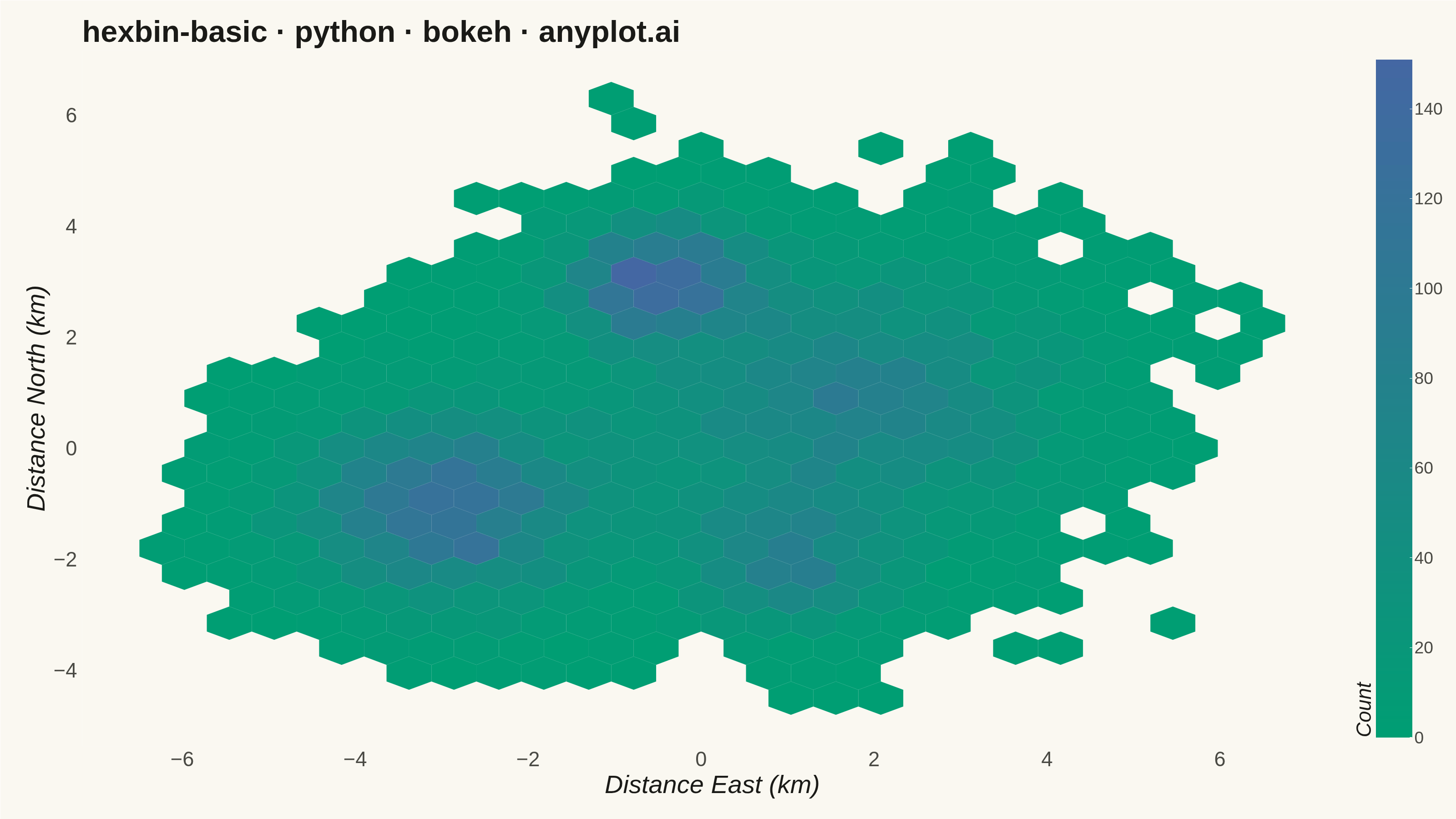
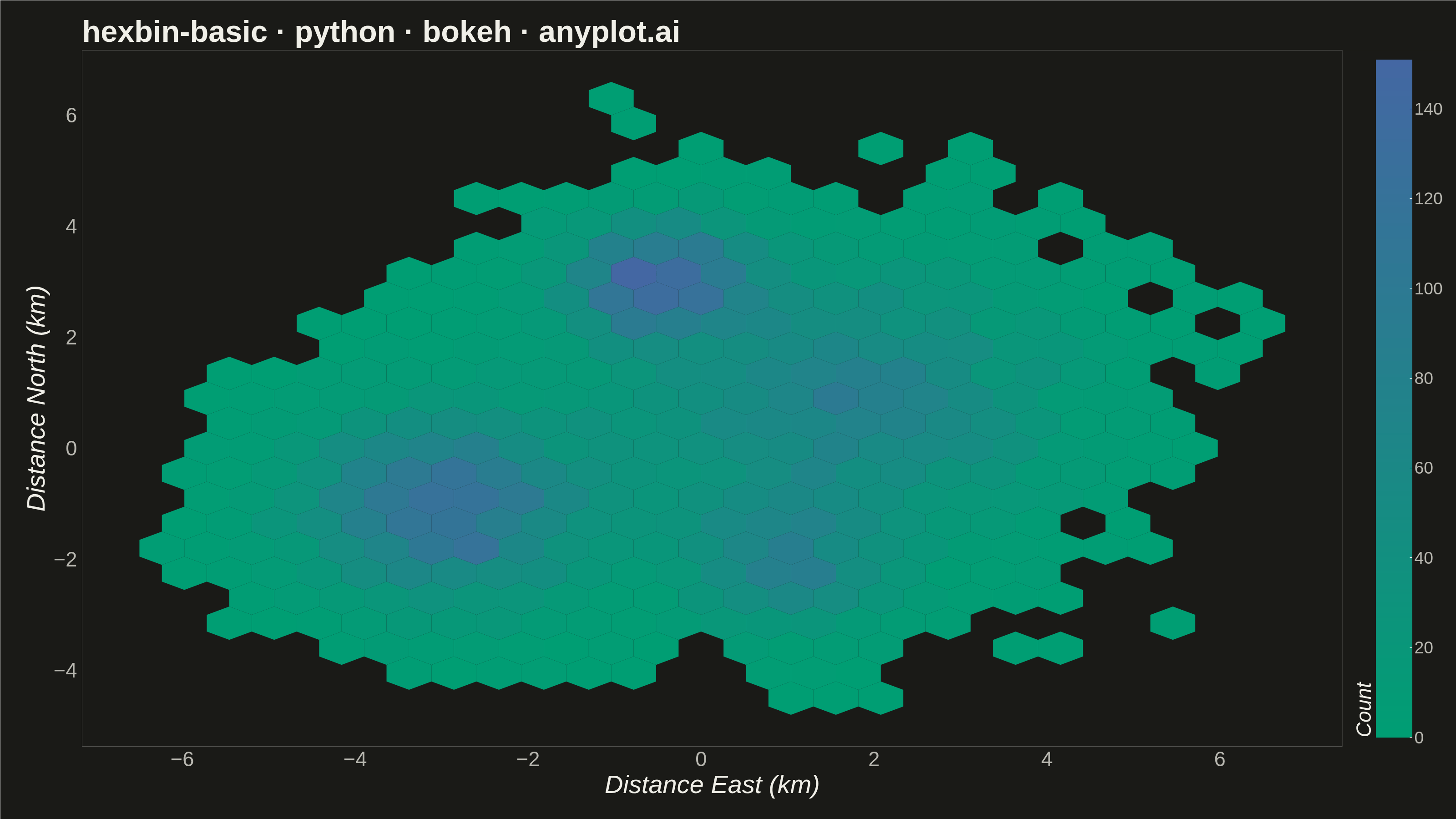
A hexagonal binning plot that visualizes the density of 2D point data by aggregating points into hexagonal bins. The color intensity of each hexagon represents the count of points within it, making it ideal for revealing density patterns in large datasets where traditional scatter plots would show overlapping points. Hexagonal bins provide better visual representation than square pixels due to their isotropy (equal distance to neighboring cells in all directions).
""" anyplot.ai
hexbin-basic: Basic Hexbin Plot
Library: bokeh 3.9.0 | Python 3.13.13
Quality: 94/100 | Created: 2026-05-29
"""

import os
import sys
import time
from pathlib import Path


# Prevent this file (bokeh.py) from shadowing the installed bokeh package
_script_dir = os.path.dirname(os.path.abspath(__file__))
sys.path = [p for p in sys.path if os.path.abspath(p) != _script_dir]

import numpy as np
from bokeh.io import output_file, save
from bokeh.models import ColorBar, ColumnDataSource, LinearColorMapper
from bokeh.plotting import figure
from bokeh.transform import transform
from bokeh.util.hex import hexbin
from PIL import Image as _PILImage
from selenium import webdriver
from selenium.webdriver.chrome.options import Options


# Theme tokens
THEME = os.getenv("ANYPLOT_THEME", "light")
PAGE_BG = "#FAF8F1" if THEME == "light" else "#1A1A17"
INK = "#1A1A17" if THEME == "light" else "#F0EFE8"
INK_SOFT = "#4A4A44" if THEME == "light" else "#B8B7B0"

# Imprint sequential colormap — green (#009E73) → blue (#4467A3), single-polarity
_c0 = (0x00, 0x9E, 0x73)
_c1 = (0x44, 0x67, 0xA3)
ANYPLOT_SEQ256 = [
    "#{:02X}{:02X}{:02X}".format(
        int(round(_c0[0] + (_c1[0] - _c0[0]) * t / 255.0)),
        int(round(_c0[1] + (_c1[1] - _c0[1]) * t / 255.0)),
        int(round(_c0[2] + (_c1[2] - _c0[2]) * t / 255.0)),
    )
    for t in range(256)
]

# Data — IoT sensor readings across urban monitoring zones (overlapping plumes)
np.random.seed(42)

centers = [(-3, -1), (2, 1), (-0.5, 3), (1.0, -2), (0.5, 0.5)]
cluster_sizes = [3500, 3000, 1800, 1200, 1500]
spreads = [1.0, 1.3, 0.65, 0.75, 1.6]

x_data, y_data = [], []
for (cx, cy), size, sigma in zip(centers, cluster_sizes, spreads, strict=True):
    x_data.extend(np.random.randn(size) * sigma + cx)
    y_data.extend(np.random.randn(size) * sigma + cy)

x = np.array(x_data)
y = np.array(y_data)

# Hexbin aggregation using Bokeh's native utility (returns HexBinResult namedtuple)
bins = hexbin(x, y, 0.3)
counts_max = int(max(bins.counts))
source = ColumnDataSource({"q": bins.q, "r": bins.r, "counts": bins.counts})

# Title — 40 chars < 67 baseline, so fontsize stays at 50pt default
title = "hexbin-basic · python · bokeh · anyplot.ai"

# Plot
p = figure(
    width=3200,
    height=1800,
    title=title,
    x_axis_label="Distance East (km)",
    y_axis_label="Distance North (km)",
    toolbar_location=None,
    min_border_bottom=160,
    min_border_left=180,
    min_border_top=110,
    min_border_right=250,
)

# Imprint sequential color mapper
mapper = LinearColorMapper(palette=ANYPLOT_SEQ256, low=0, high=counts_max)

# Hex tiles
p.hex_tile(q="q", r="r", size=0.3, line_color=None, source=source, fill_color=transform("counts", mapper))

# Color bar
color_bar = ColorBar(
    color_mapper=mapper,
    width=80,
    title="Count",
    title_text_font_size="34pt",
    title_text_color=INK,
    major_label_text_font_size="28pt",
    major_label_text_color=INK_SOFT,
    background_fill_color=PAGE_BG,
    background_fill_alpha=1.0,
    padding=20,
)
p.add_layout(color_bar, "right")

# Chrome — theme-adaptive
p.background_fill_color = PAGE_BG
p.border_fill_color = PAGE_BG
p.outline_line_color = None

p.title.text_font_size = "50pt"
p.title.text_color = INK
p.title.text_font_style = "bold"

p.xaxis.axis_label_text_font_size = "42pt"
p.yaxis.axis_label_text_font_size = "42pt"
p.xaxis.major_label_text_font_size = "34pt"
p.yaxis.major_label_text_font_size = "34pt"

p.xaxis.axis_label_text_color = INK
p.yaxis.axis_label_text_color = INK
p.xaxis.major_label_text_color = INK_SOFT
p.yaxis.major_label_text_color = INK_SOFT

p.xaxis.axis_line_color = None
p.yaxis.axis_line_color = None
p.xaxis.major_tick_line_color = None
p.yaxis.major_tick_line_color = None
p.xaxis.minor_tick_line_color = None
p.yaxis.minor_tick_line_color = None

p.grid.visible = False

# Save HTML (interactive catalog artifact)
output_file(f"plot-{THEME}.html")
save(p)

# Screenshot via Selenium headless Chrome
# --window-size alone is eaten by Chrome chrome in headless mode (gives 1661 instead of 1800)
W, H = 3200, 1800
opts = Options()
for arg in (
    "--headless=new",
    "--no-sandbox",
    "--disable-dev-shm-usage",
    "--disable-gpu",
    f"--window-size={W},{H}",
    "--hide-scrollbars",
):
    opts.add_argument(arg)
driver = webdriver.Chrome(options=opts)
driver.execute_cdp_cmd(
    "Emulation.setDeviceMetricsOverride", {"width": W, "height": H, "deviceScaleFactor": 1, "mobile": False}
)
driver.get(f"file://{Path(f'plot-{THEME}.html').resolve()}")
time.sleep(3)
driver.save_screenshot(f"plot-{THEME}.png")
driver.quit()

# Belt-and-braces: pin the saved PNG to exact dims so the post-render gate passes
_img = _PILImage.open(f"plot-{THEME}.png").convert("RGB")
if _img.size != (W, H):
    _norm = _PILImage.new("RGB", (W, H), PAGE_BG)
    _norm.paste(_img, ((W - _img.size[0]) // 2, (H - _img.size[1]) // 2))
    _norm.save(f"plot-{THEME}.png")
Runnable source as JSON, for any HTTP client: https://api.anyplot.ai/specs/hexbin-basic/bokeh/code. Any spec id and library id listed in llms-full.txt fit the same URL shape; every URL below is complete and callable.
{
  "spec_id": "hexbin-basic",
  "language": "python",
  "library": "bokeh",
  "page": "https://anyplot.ai/hexbin-basic/python/bokeh",
  "hub": "https://anyplot.ai/hexbin-basic",
  "code_json": "https://api.anyplot.ai/specs/hexbin-basic/bokeh/code",
  "spec_json": "https://api.anyplot.ai/specs/hexbin-basic",
  "render_light_png": "https://storage.googleapis.com/anyplot-images/plots/hexbin-basic/python/bokeh/plot-light.png",
  "render_dark_png": "https://storage.googleapis.com/anyplot-images/plots/hexbin-basic/python/bokeh/plot-dark.png",
  "interactive_light_html": "https://storage.googleapis.com/anyplot-images/plots/hexbin-basic/python/bokeh/plot-light.html",
  "interactive_dark_html": "https://storage.googleapis.com/anyplot-images/plots/hexbin-basic/python/bokeh/plot-dark.html",
  "quality_score": 94.0,
  "license": "MIT",
  "guide": "https://anyplot.ai/llms.txt"
}
Part of Basic Hexbin Plot on anyplot.ai.