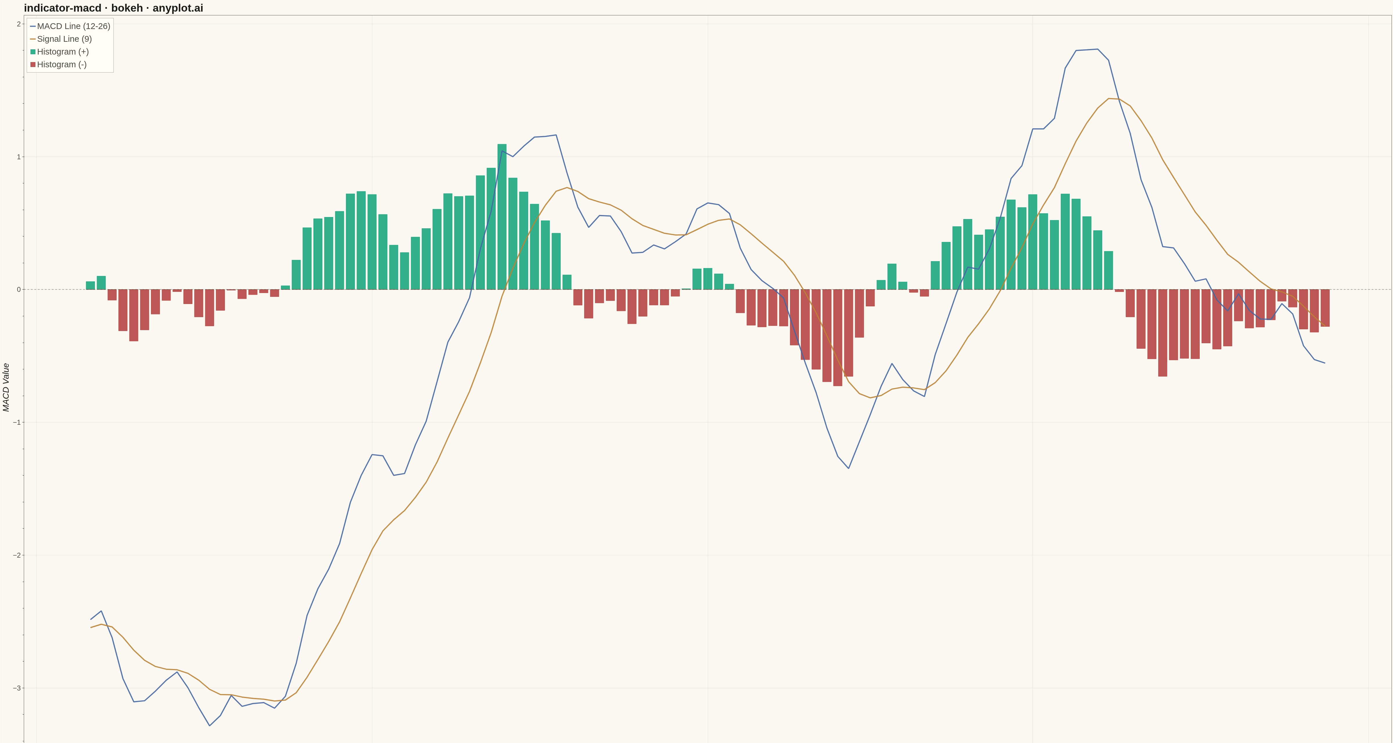
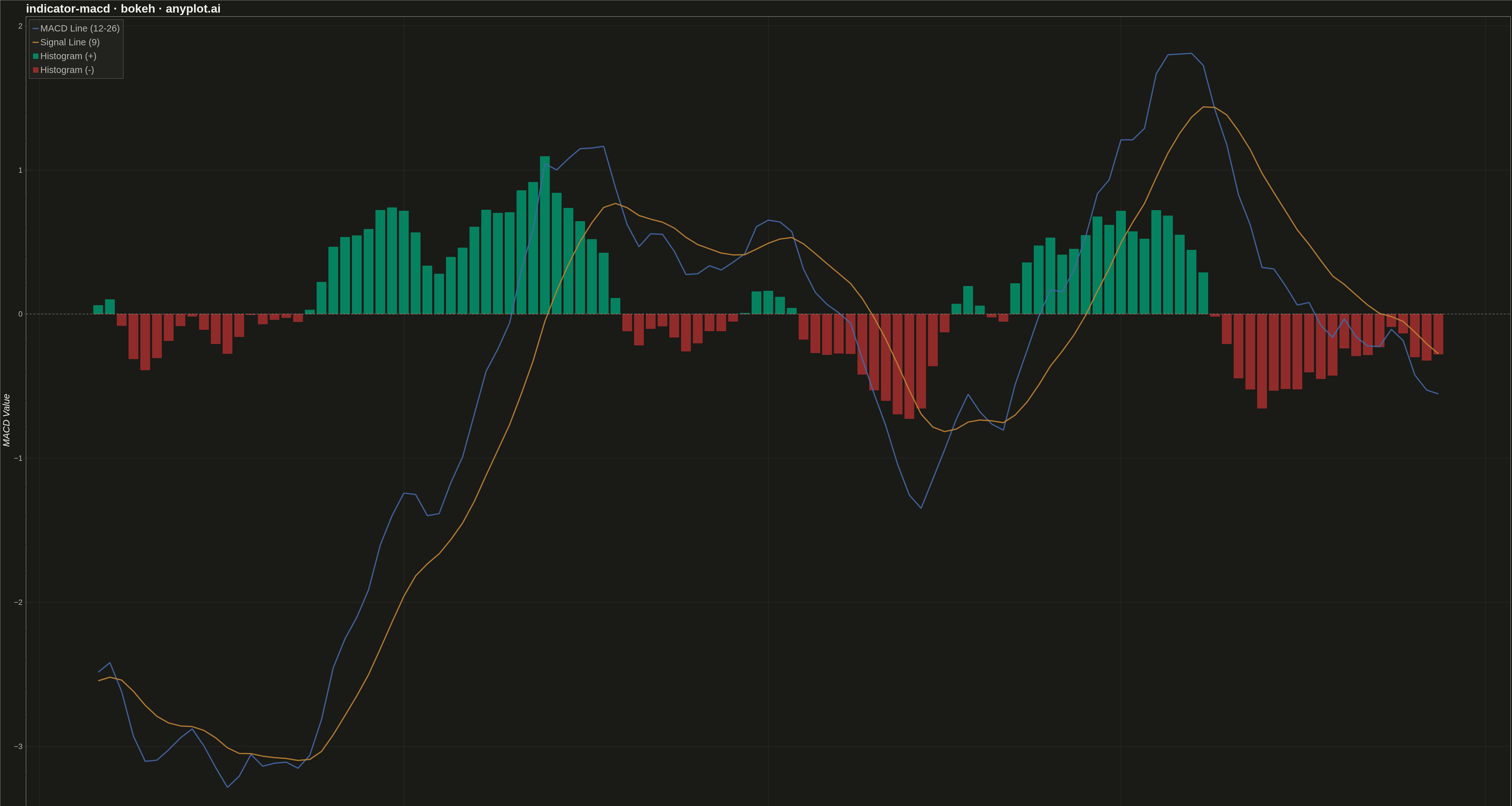
A MACD (Moving Average Convergence Divergence) chart displaying three components: the MACD line, signal line, and histogram. The MACD line represents the difference between 12-day and 26-day exponential moving averages, while the signal line is a 9-day EMA of the MACD. The histogram visualizes the difference between these two lines. This is an essential momentum oscillator for technical analysis, helping traders identify trend direction, momentum strength, and potential buy/sell signals through line crossovers.
""" anyplot.ai
indicator-macd: MACD Technical Indicator Chart
Library: bokeh 3.9.0 | Python 3.13.13
Quality: 88/100 | Updated: 2026-05-16
"""

import os
import time
from pathlib import Path

import numpy as np
import pandas as pd
from bokeh.io import output_file, save
from bokeh.models import ColumnDataSource, HoverTool, Legend, Span
from bokeh.plotting import figure
from selenium import webdriver
from selenium.webdriver.chrome.options import Options


# Theme tokens
THEME = os.getenv("ANYPLOT_THEME", "light")
PAGE_BG = "#FAF8F1" if THEME == "light" else "#1A1A17"
ELEVATED_BG = "#FFFDF6" if THEME == "light" else "#242420"
INK = "#1A1A17" if THEME == "light" else "#F0EFE8"
INK_SOFT = "#4A4A44" if THEME == "light" else "#B8B7B0"

# Okabe-Ito palette for MACD components
HIST_POSITIVE = "#009E73"  # Position 1 - brand green
HIST_NEGATIVE = "#AE3030"  # imprint red — bars below zero
MACD_LINE_COLOR = "#4467A3"  # Position 3 - blue
SIGNAL_LINE_COLOR = "#BD8233"  # imprint ochre — distinct from histogram bars

# Data - Generate synthetic stock price data and calculate MACD
np.random.seed(42)
n_days = 150

# Generate realistic price movement with trend and volatility
returns = np.random.normal(0.001, 0.02, n_days)
price = 100 * np.cumprod(1 + returns)

# Calculate EMAs
df = pd.DataFrame({"date": pd.date_range("2025-06-01", periods=n_days, freq="D"), "close": price})

# Calculate 12-day and 26-day EMA
df["ema12"] = df["close"].ewm(span=12, adjust=False).mean()
df["ema26"] = df["close"].ewm(span=26, adjust=False).mean()

# Calculate MACD line (12-day EMA - 26-day EMA)
df["macd"] = df["ema12"] - df["ema26"]

# Calculate signal line (9-day EMA of MACD)
df["signal"] = df["macd"].ewm(span=9, adjust=False).mean()

# Calculate histogram (MACD - Signal)
df["histogram"] = df["macd"] - df["signal"]

# Use data from day 35 onwards for meaningful MACD values
df = df.iloc[35:].reset_index(drop=True)

# Separate positive and negative histogram values for coloring
df["hist_positive"] = df["histogram"].where(df["histogram"] >= 0, 0)
df["hist_negative"] = df["histogram"].where(df["histogram"] < 0, 0)

# Format date for display
df["date_str"] = df["date"].dt.strftime("%Y-%m-%d")

# Create ColumnDataSource
source = ColumnDataSource(
    data={
        "date": df["date"],
        "date_str": df["date_str"],
        "macd": df["macd"],
        "signal": df["signal"],
        "histogram": df["histogram"],
        "hist_positive": df["hist_positive"],
        "hist_negative": df["hist_negative"],
    }
)

# Plot
p = figure(
    width=4800,
    height=2700,
    x_axis_type="datetime",
    title="indicator-macd · bokeh · anyplot.ai",
    x_axis_label="Date",
    y_axis_label="MACD Value",
)

# Calculate bar width (1 day in milliseconds, slightly narrower for gaps)
bar_width = 0.8 * 24 * 60 * 60 * 1000

# Plot histogram bars - positive (Okabe-Ito green)
hist_pos = p.vbar(
    x="date",
    top="hist_positive",
    width=bar_width,
    source=source,
    fill_color=HIST_POSITIVE,
    line_color=HIST_POSITIVE,
    line_width=1,
    alpha=0.8,
)

# Plot histogram bars - negative (Okabe-Ito orange)
hist_neg = p.vbar(
    x="date",
    top="hist_negative",
    width=bar_width,
    source=source,
    fill_color=HIST_NEGATIVE,
    line_color=HIST_NEGATIVE,
    line_width=1,
    alpha=0.8,
)

# Plot MACD line (Okabe-Ito blue)
macd_line = p.line(x="date", y="macd", source=source, line_color=MACD_LINE_COLOR, line_width=4, alpha=0.9)

# Plot signal line (Okabe-Ito orange)
signal_line = p.line(x="date", y="signal", source=source, line_color=SIGNAL_LINE_COLOR, line_width=4, alpha=0.9)

# Add zero reference line
zero_line = Span(location=0, dimension="width", line_color=INK_SOFT, line_dash="dashed", line_width=2, line_alpha=0.5)
p.add_layout(zero_line)

# Create legend
legend = Legend(
    items=[
        ("MACD Line (12-26)", [macd_line]),
        ("Signal Line (9)", [signal_line]),
        ("Histogram (+)", [hist_pos]),
        ("Histogram (-)", [hist_neg]),
    ],
    location="top_left",
)
legend.label_text_font_size = "22pt"
legend.spacing = 10
legend.background_fill_color = ELEVATED_BG
legend.background_fill_alpha = 0.9
legend.border_line_color = INK_SOFT
legend.label_text_color = INK_SOFT
p.add_layout(legend)

# Add HoverTool for interactivity
hover = HoverTool(
    tooltips=[
        ("Date", "@date_str"),
        ("MACD", "@macd{0.000}"),
        ("Signal", "@signal{0.000}"),
        ("Histogram", "@histogram{0.000}"),
    ]
)
p.add_tools(hover)

# Style
p.title.text_font_size = "28pt"
p.title.text_color = INK

p.xaxis.axis_label_text_font_size = "22pt"
p.yaxis.axis_label_text_font_size = "22pt"
p.xaxis.axis_label_text_color = INK
p.yaxis.axis_label_text_color = INK

p.xaxis.major_label_text_font_size = "18pt"
p.yaxis.major_label_text_font_size = "18pt"
p.xaxis.major_label_text_color = INK_SOFT
p.yaxis.major_label_text_color = INK_SOFT

# Grid styling - subtle
p.xgrid.grid_line_alpha = 0.10
p.ygrid.grid_line_alpha = 0.10
p.xgrid.grid_line_color = INK
p.ygrid.grid_line_color = INK

# Backgrounds and borders (theme-adaptive)
p.background_fill_color = PAGE_BG
p.border_fill_color = PAGE_BG
p.outline_line_color = INK_SOFT
p.outline_line_width = 1

# Axis styling
p.xaxis.axis_line_color = INK_SOFT
p.yaxis.axis_line_color = INK_SOFT
p.xaxis.axis_line_width = 1
p.yaxis.axis_line_width = 1
p.xaxis.major_tick_line_color = INK_SOFT
p.yaxis.major_tick_line_color = INK_SOFT

# Hide toolbar
p.toolbar_location = None

# Save HTML
output_file(f"plot-{THEME}.html")
save(p)

# Screenshot with headless Chrome
W, H = 4800, 2700
opts = Options()
for arg in (
    "--headless=new",
    "--no-sandbox",
    "--disable-dev-shm-usage",
    "--disable-gpu",
    f"--window-size={W},{H}",
    "--hide-scrollbars",
):
    opts.add_argument(arg)
driver = webdriver.Chrome(options=opts)
driver.set_window_size(W, H)
driver.get(f"file://{Path(f'plot-{THEME}.html').resolve()}")
time.sleep(3)  # let bokeh's JS render the canvas
driver.save_screenshot(f"plot-{THEME}.png")
driver.quit()
Runnable source as JSON, for any HTTP client: https://api.anyplot.ai/specs/indicator-macd/bokeh/code. Any spec id and library id listed in llms-full.txt fit the same URL shape; every URL below is complete and callable.
{
  "spec_id": "indicator-macd",
  "language": "python",
  "library": "bokeh",
  "page": "https://anyplot.ai/indicator-macd/python/bokeh",
  "hub": "https://anyplot.ai/indicator-macd",
  "code_json": "https://api.anyplot.ai/specs/indicator-macd/bokeh/code",
  "spec_json": "https://api.anyplot.ai/specs/indicator-macd",
  "render_light_png": "https://storage.googleapis.com/anyplot-images/plots/indicator-macd/python/bokeh/plot-light.png",
  "render_dark_png": "https://storage.googleapis.com/anyplot-images/plots/indicator-macd/python/bokeh/plot-dark.png",
  "interactive_light_html": "https://storage.googleapis.com/anyplot-images/plots/indicator-macd/python/bokeh/plot-light.html",
  "interactive_dark_html": "https://storage.googleapis.com/anyplot-images/plots/indicator-macd/python/bokeh/plot-dark.html",
  "quality_score": 88.0,
  "license": "MIT",
  "guide": "https://anyplot.ai/llms.txt"
}
Part of MACD Technical Indicator Chart on anyplot.ai.