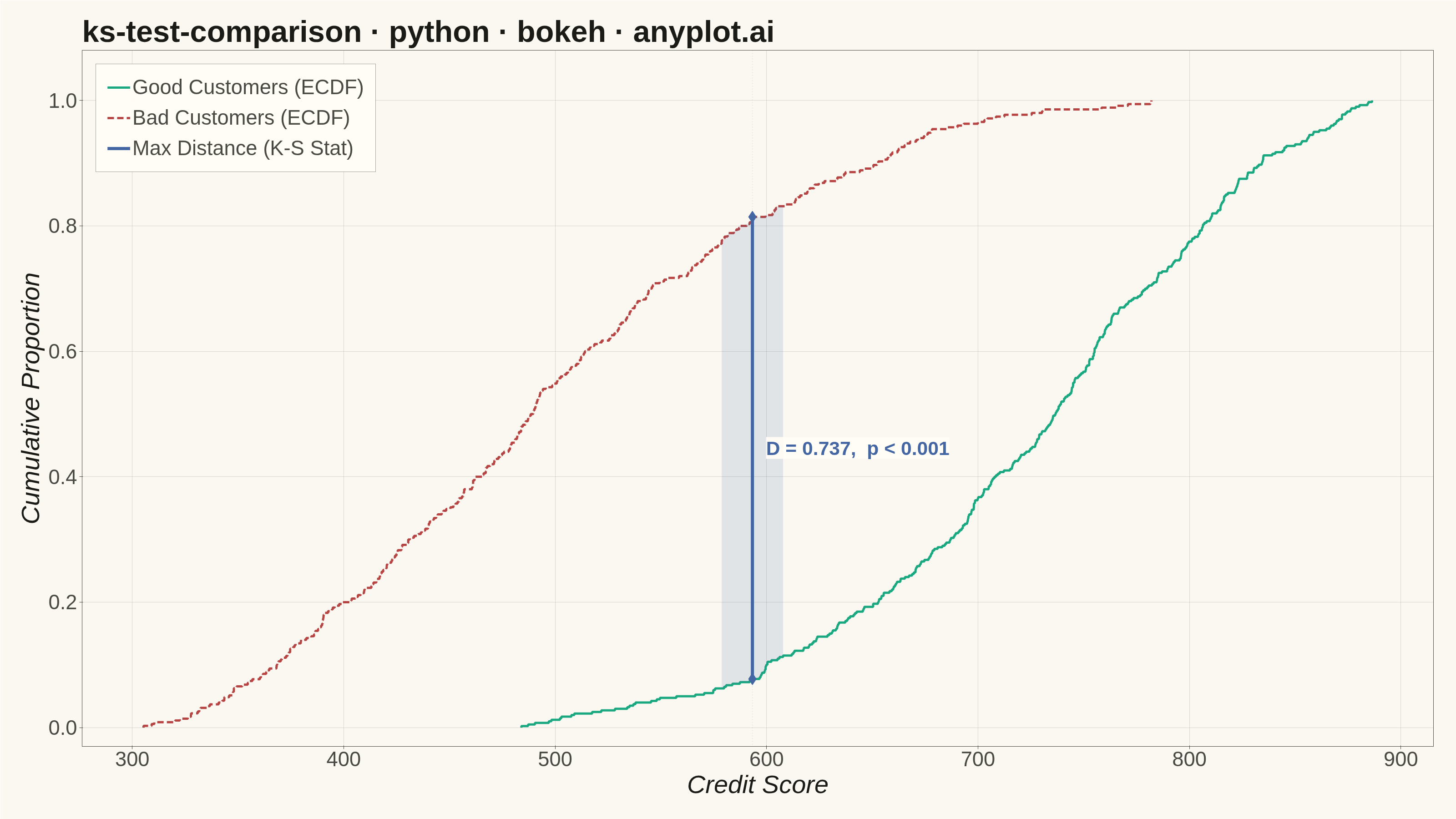
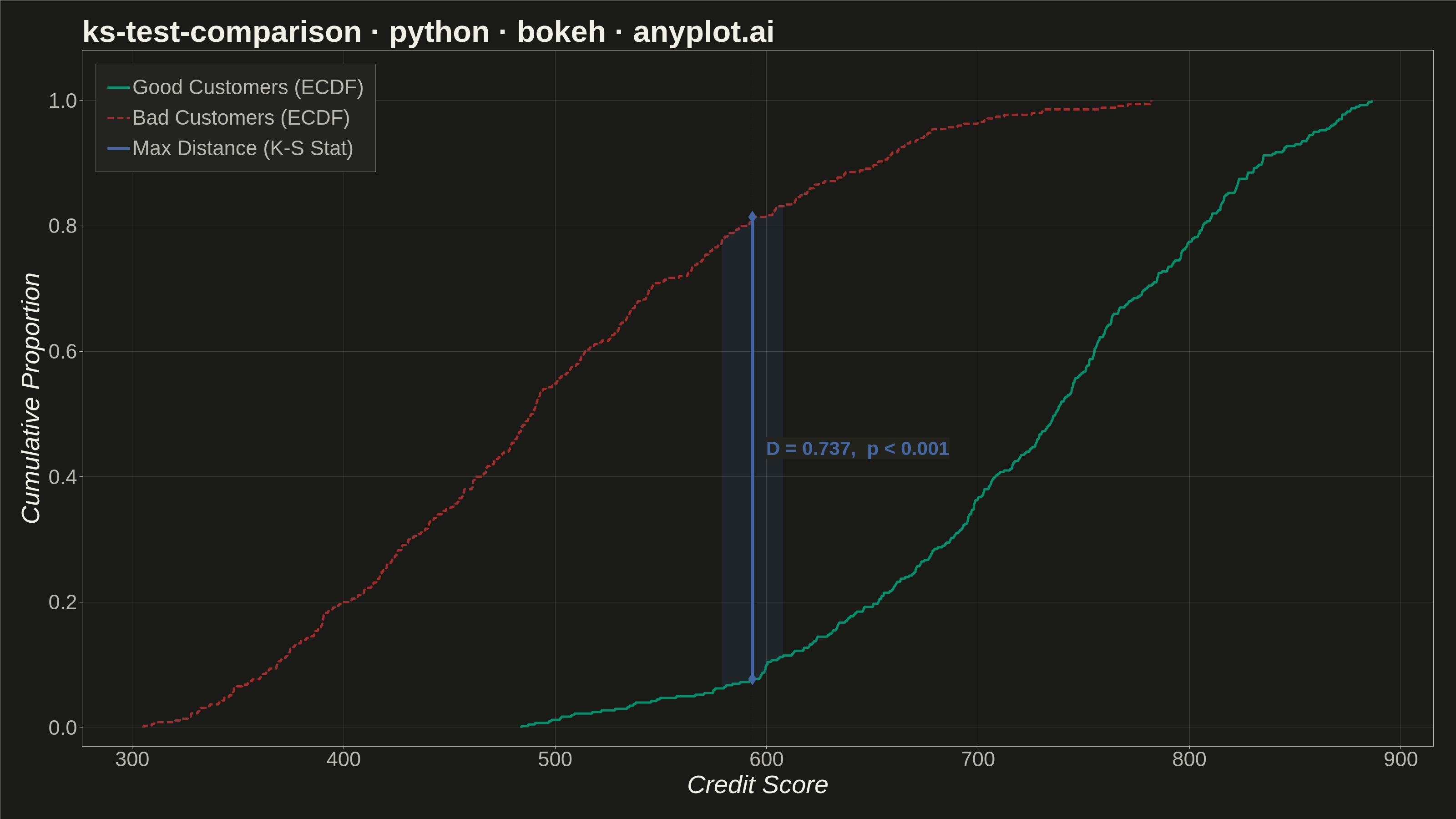
A Kolmogorov-Smirnov (K-S) plot compares two empirical cumulative distribution functions (ECDFs) and visualizes the K-S statistic, which is the maximum vertical distance between the two distributions. The plot displays both ECDFs as step functions, highlights the point of maximum divergence, and typically reports the K-S statistic value and p-value for hypothesis testing. This visualization is essential for determining whether two samples come from the same underlying distribution.
""" anyplot.ai
ks-test-comparison: Kolmogorov-Smirnov Plot for Distribution Comparison
Library: bokeh 3.9.0 | Python 3.13.13
Quality: 92/100 | Updated: 2026-05-29
"""

import os
import sys
import time
from pathlib import Path


# bokeh.py is the script name — remove its directory from sys.path so that
# `import bokeh` resolves to the installed package, not this file itself.
_here = os.path.dirname(os.path.abspath(__file__))
sys.path[:] = [p for p in sys.path if os.path.abspath(p) != _here]

import numpy as np
from bokeh.io import output_file, save
from bokeh.models import (
    Band,
    ColumnDataSource,
    HoverTool,
    Label,
    Legend,
    LegendItem,
    NumeralTickFormatter,
    Range1d,
    Span,
)
from bokeh.plotting import figure
from scipy import stats
from selenium import webdriver
from selenium.webdriver.chrome.options import Options


# Theme tokens (Imprint palette — theme-adaptive chrome)
THEME = os.getenv("ANYPLOT_THEME", "light")
PAGE_BG = "#FAF8F1" if THEME == "light" else "#1A1A17"
ELEVATED_BG = "#FFFDF6" if THEME == "light" else "#242420"
INK = "#1A1A17" if THEME == "light" else "#F0EFE8"
INK_SOFT = "#4A4A44" if THEME == "light" else "#B8B7B0"

# Imprint categorical palette — semantic assignment: Good=green, Bad=red, KS=blue
COLOR_GOOD = "#009E73"  # position 1, brand green — semantic: good/pass
COLOR_BAD = "#AE3030"  # position 5, matte red — semantic: bad/fail
COLOR_KS = "#4467A3"  # position 3, blue — neutral emphasis for the distance measurement

# Data — Credit scoring: Good vs Bad customer score distributions
np.random.seed(42)
good_scores = np.random.beta(5, 2, 400) * 600 + 300  # Good customers: higher scores
bad_scores = np.random.beta(2, 4, 350) * 600 + 300  # Bad customers: lower scores

# Compute ECDFs
good_sorted = np.sort(good_scores)
good_ecdf = np.arange(1, len(good_sorted) + 1) / len(good_sorted)
bad_sorted = np.sort(bad_scores)
bad_ecdf = np.arange(1, len(bad_sorted) + 1) / len(bad_sorted)

# K-S test
ks_stat, p_value = stats.ks_2samp(good_scores, bad_scores)

# Find point of maximum divergence
all_values = np.sort(np.concatenate([good_scores, bad_scores]))
good_ecdf_at = np.searchsorted(good_sorted, all_values, side="right") / len(good_sorted)
bad_ecdf_at = np.searchsorted(bad_sorted, all_values, side="right") / len(bad_sorted)
max_idx = np.argmax(np.abs(good_ecdf_at - bad_ecdf_at))
max_x = all_values[max_idx]
max_y_good = good_ecdf_at[max_idx]
max_y_bad = bad_ecdf_at[max_idx]
ks_y_lower = min(max_y_good, max_y_bad)
ks_y_upper = max(max_y_good, max_y_bad)

# Build step function arrays — interleave x,y pairs for step rendering
good_x_step = np.concatenate([[good_sorted[0]], np.repeat(good_sorted, 2)[1:]])
good_y_step = np.concatenate([[0], np.repeat(good_ecdf, 2)[:-1]])
bad_x_step = np.concatenate([[bad_sorted[0]], np.repeat(bad_sorted, 2)[1:]])
bad_y_step = np.concatenate([[0], np.repeat(bad_ecdf, 2)[:-1]])

good_source = ColumnDataSource(data={"x": good_x_step, "y": good_y_step})
bad_source = ColumnDataSource(data={"x": bad_x_step, "y": bad_y_step})

# Shaded band near max divergence for visual storytelling (distinctive Bokeh Band model)
band_mask = (all_values >= max_x - 15) & (all_values <= max_x + 15)
band_x = all_values[band_mask]
band_upper = np.maximum(good_ecdf_at[band_mask], bad_ecdf_at[band_mask])
band_lower = np.minimum(good_ecdf_at[band_mask], bad_ecdf_at[band_mask])
band_source = ColumnDataSource(data={"x": band_x, "upper": band_upper, "lower": band_lower})

# Plot — canonical 3200×1800 landscape canvas; toolbar_location=None avoids toolbar height offset
title = "ks-test-comparison · python · bokeh · anyplot.ai"
p = figure(
    width=3200,
    height=1800,
    title=title,
    x_axis_label="Credit Score",
    y_axis_label="Cumulative Proportion",
    y_range=Range1d(-0.03, 1.08),
    toolbar_location=None,
    min_border_bottom=160,
    min_border_left=180,
    min_border_top=110,
    min_border_right=50,
)

# Shaded band between ECDFs at max divergence
band = Band(
    base="x", upper="upper", lower="lower", source=band_source, fill_color=COLOR_KS, fill_alpha=0.14, line_color=None
)
p.add_layout(band)

# ECDF step lines — solid green (Good) vs dashed red (Bad)
good_line = p.line(x="x", y="y", source=good_source, line_width=5, line_color=COLOR_GOOD, alpha=0.9)
bad_line = p.line(x="x", y="y", source=bad_source, line_width=5, line_color=COLOR_BAD, alpha=0.9, line_dash=[14, 7])

# HoverTool for HTML artifact — shows exact ECDF values at cursor position
hover = HoverTool(tooltips=[("Score", "@x{0.0}"), ("Cum. Proportion", "@y{0.000}")], renderers=[good_line, bad_line])
p.add_tools(hover)

# K-S segment — vertical line at maximum divergence
ks_segment_source = ColumnDataSource(data={"x0": [max_x], "y0": [ks_y_lower], "x1": [max_x], "y1": [ks_y_upper]})
ks_line = p.segment(x0="x0", y0="y0", x1="x1", y1="y1", source=ks_segment_source, line_width=7, line_color=COLOR_KS)

# Diamond markers at K-S segment endpoints
ks_marker_source = ColumnDataSource(data={"x": [max_x, max_x], "y": [ks_y_lower, ks_y_upper]})
p.scatter(x="x", y="y", source=ks_marker_source, size=26, color=COLOR_KS, marker="diamond")

# Annotation — K-S statistic and p-value, prominently sized with theme-adaptive background
p_text = "p < 0.001" if p_value < 0.001 else f"p = {p_value:.4f}"
ks_label = Label(
    x=max_x,
    y=(ks_y_lower + ks_y_upper) / 2,
    text=f"D = {ks_stat:.3f},  {p_text}",
    text_font_size="32pt",
    text_color=COLOR_KS,
    text_font_style="bold",
    text_baseline="middle",
    x_offset=30,
    background_fill_color=ELEVATED_BG,
    background_fill_alpha=0.92,
)
p.add_layout(ks_label)

# Subtle vertical reference line at max divergence
max_div_span = Span(
    location=max_x, dimension="height", line_color=COLOR_KS, line_alpha=0.12, line_width=2, line_dash="dotted"
)
p.add_layout(max_div_span)

# Legend — canonical 34pt size from bokeh.md, theme-adaptive fill
legend = Legend(
    items=[
        LegendItem(label="Good Customers (ECDF)", renderers=[good_line]),
        LegendItem(label="Bad Customers (ECDF)", renderers=[bad_line]),
        LegendItem(label="Max Distance (K-S Stat)", renderers=[ks_line]),
    ],
    location="top_left",
)
legend.label_text_font_size = "34pt"
legend.label_text_color = INK_SOFT
legend.background_fill_color = ELEVATED_BG
legend.border_line_color = INK_SOFT
legend.glyph_height = 40
legend.glyph_width = 50
legend.padding = 25
legend.spacing = 15
legend.margin = 30
p.add_layout(legend, "center")

# Typography — canonical bokeh.md sizes; title is 49 chars < 67, so no scaling needed
p.title.text_font_size = "50pt"
p.title.text_font_style = "bold"
p.title.text_color = INK

p.xaxis.axis_label_text_font_size = "42pt"
p.yaxis.axis_label_text_font_size = "42pt"
p.xaxis.axis_label_text_color = INK
p.yaxis.axis_label_text_color = INK
p.xaxis.major_label_text_font_size = "34pt"
p.yaxis.major_label_text_font_size = "34pt"
p.xaxis.major_label_text_color = INK_SOFT
p.yaxis.major_label_text_color = INK_SOFT

# Theme-adaptive chrome
p.background_fill_color = PAGE_BG
p.border_fill_color = PAGE_BG
p.outline_line_color = INK_SOFT

p.xaxis.axis_line_color = INK_SOFT
p.yaxis.axis_line_color = INK_SOFT
p.xaxis.minor_tick_line_color = None
p.yaxis.minor_tick_line_color = None
p.xaxis.major_tick_line_color = INK_SOFT
p.yaxis.major_tick_line_color = INK_SOFT

p.xgrid.grid_line_color = INK
p.ygrid.grid_line_color = INK
p.xgrid.grid_line_alpha = 0.15
p.ygrid.grid_line_alpha = 0.15

p.yaxis.formatter = NumeralTickFormatter(format="0.0")

# Save HTML (interactive catalog artifact)
output_file(f"plot-{THEME}.html")
save(p)

# Screenshot with headless Selenium — Selenium 4 / Selenium Manager resolves the driver.
# Use CDP setDeviceMetricsOverride so the inner viewport is authoritative:
# --window-size alone is eaten by Chrome chrome in headless mode (gives 1661 instead of 1800).
W, H = 3200, 1800
opts = Options()
for arg in (
    "--headless=new",
    "--no-sandbox",
    "--disable-dev-shm-usage",
    "--disable-gpu",
    f"--window-size={W},{H}",
    "--hide-scrollbars",
):
    opts.add_argument(arg)
driver = webdriver.Chrome(options=opts)
driver.execute_cdp_cmd(
    "Emulation.setDeviceMetricsOverride", {"width": W, "height": H, "deviceScaleFactor": 1, "mobile": False}
)
driver.get(f"file://{Path(f'plot-{THEME}.html').resolve()}")
time.sleep(3)
driver.save_screenshot(f"plot-{THEME}.png")
driver.quit()

# Belt-and-braces: pin the saved PNG to exact dims so the post-render gate passes
from PIL import Image as _PILImage


_img = _PILImage.open(f"plot-{THEME}.png").convert("RGB")
if _img.size != (W, H):
    _norm = _PILImage.new("RGB", (W, H), PAGE_BG)
    _norm.paste(_img, ((W - _img.size[0]) // 2, (H - _img.size[1]) // 2))
    _norm.save(f"plot-{THEME}.png")
Runnable source as JSON, for any HTTP client: https://api.anyplot.ai/specs/ks-test-comparison/bokeh/code. Any spec id and library id listed in llms-full.txt fit the same URL shape; every URL below is complete and callable.
{
  "spec_id": "ks-test-comparison",
  "language": "python",
  "library": "bokeh",
  "page": "https://anyplot.ai/ks-test-comparison/python/bokeh",
  "hub": "https://anyplot.ai/ks-test-comparison",
  "code_json": "https://api.anyplot.ai/specs/ks-test-comparison/bokeh/code",
  "spec_json": "https://api.anyplot.ai/specs/ks-test-comparison",
  "render_light_png": "https://storage.googleapis.com/anyplot-images/plots/ks-test-comparison/python/bokeh/plot-light.png",
  "render_dark_png": "https://storage.googleapis.com/anyplot-images/plots/ks-test-comparison/python/bokeh/plot-dark.png",
  "interactive_light_html": "https://storage.googleapis.com/anyplot-images/plots/ks-test-comparison/python/bokeh/plot-light.html",
  "interactive_dark_html": "https://storage.googleapis.com/anyplot-images/plots/ks-test-comparison/python/bokeh/plot-dark.html",
  "quality_score": 92.0,
  "license": "MIT",
  "guide": "https://anyplot.ai/llms.txt"
}
Part of Kolmogorov-Smirnov Plot for Distribution Comparison on anyplot.ai.