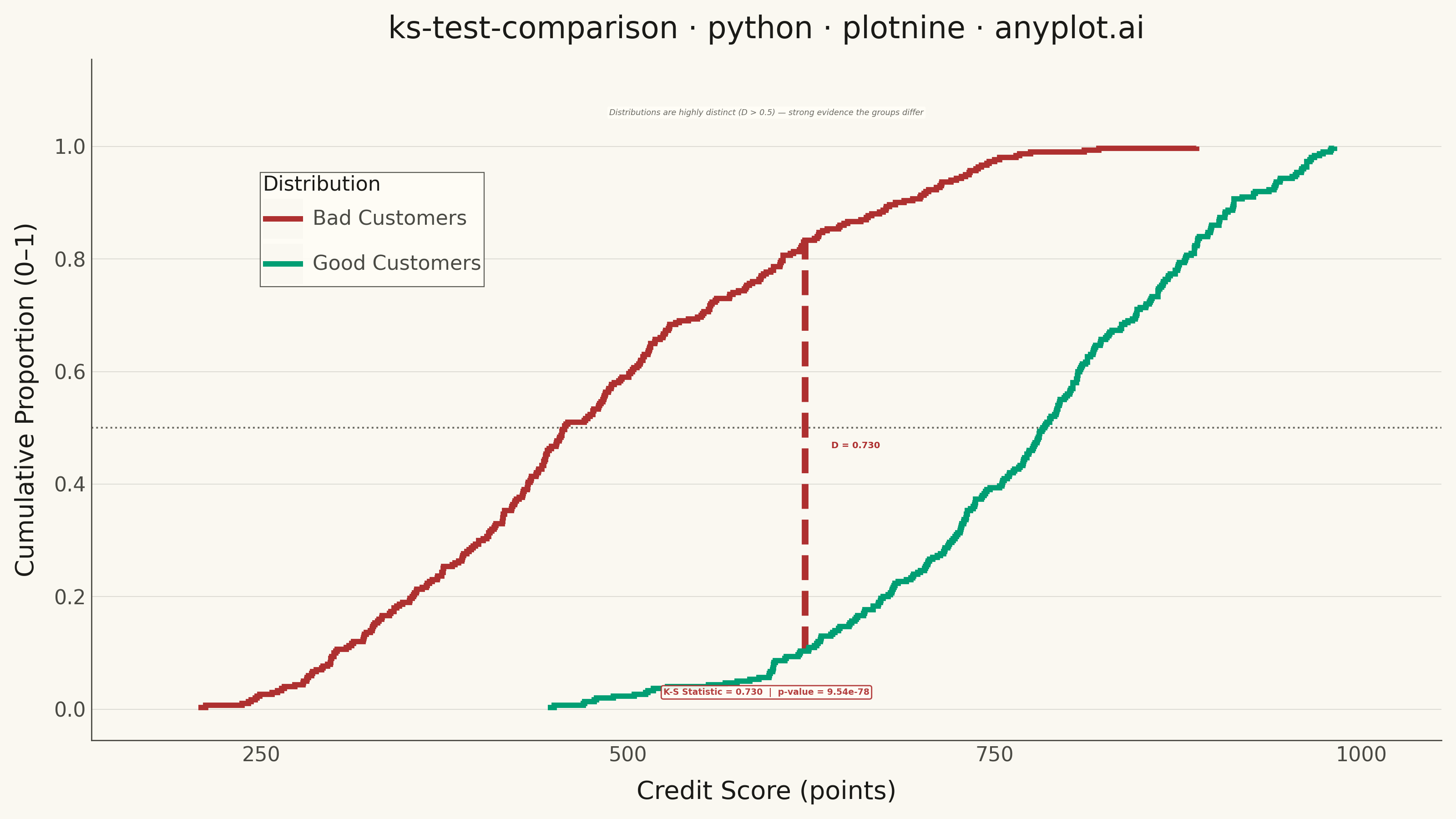
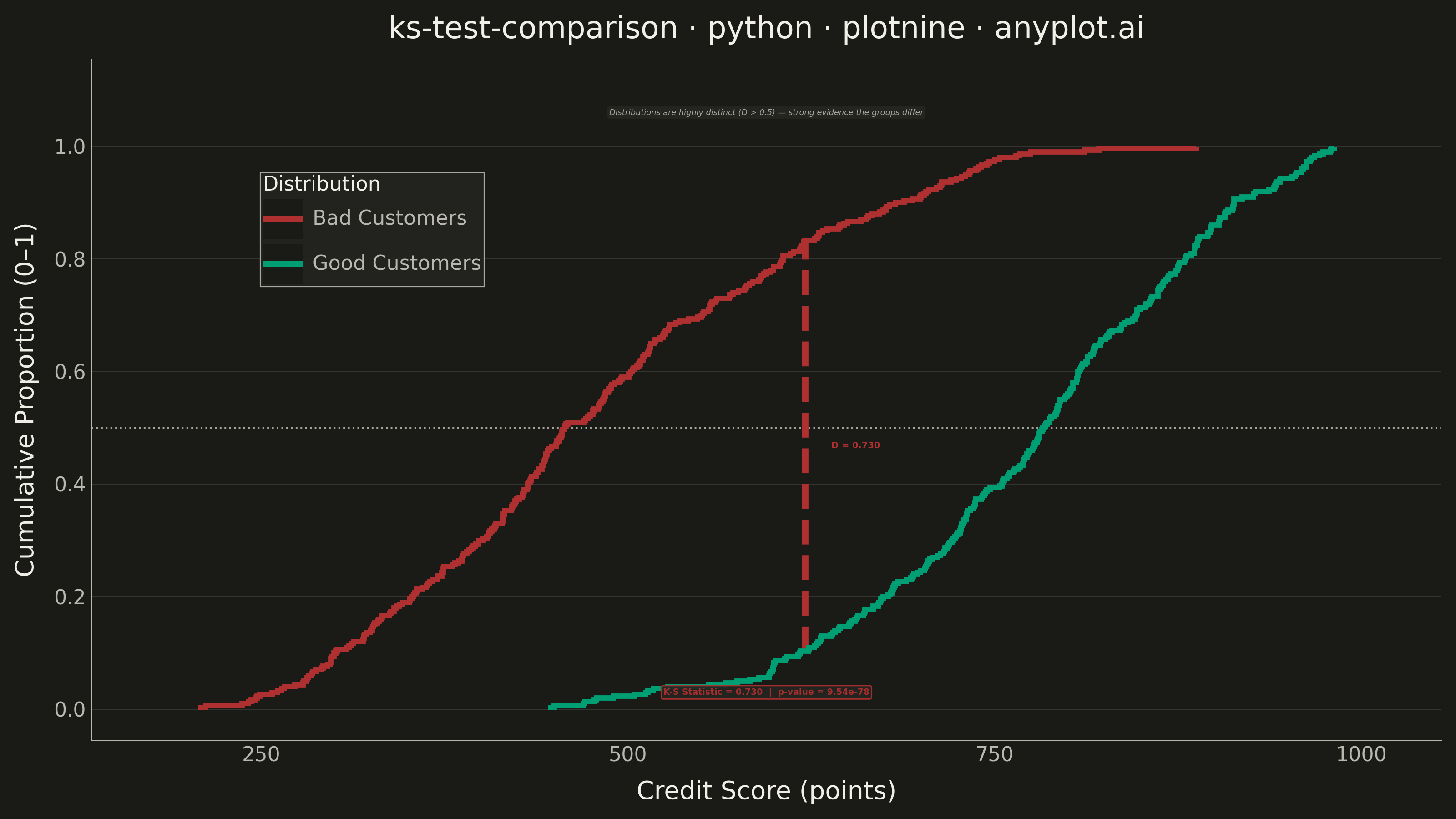
A Kolmogorov-Smirnov (K-S) plot compares two empirical cumulative distribution functions (ECDFs) and visualizes the K-S statistic, which is the maximum vertical distance between the two distributions. The plot displays both ECDFs as step functions, highlights the point of maximum divergence, and typically reports the K-S statistic value and p-value for hypothesis testing. This visualization is essential for determining whether two samples come from the same underlying distribution.
""" anyplot.ai
ks-test-comparison: Kolmogorov-Smirnov Plot for Distribution Comparison
Library: plotnine 0.15.4 | Python 3.13.13
Quality: 88/100 | Updated: 2026-05-29
"""

import os

import numpy as np
import pandas as pd
from plotnine import (
    aes,
    annotate,
    element_blank,
    element_line,
    element_rect,
    element_text,
    geom_hline,
    geom_segment,
    geom_step,
    ggplot,
    labs,
    scale_color_manual,
    scale_x_continuous,
    scale_y_continuous,
    theme,
    theme_minimal,
)
from scipy import stats


# Theme tokens — Imprint palette
THEME = os.getenv("ANYPLOT_THEME", "light")
PAGE_BG = "#FAF8F1" if THEME == "light" else "#1A1A17"
ELEVATED_BG = "#FFFDF6" if THEME == "light" else "#242420"
INK = "#1A1A17" if THEME == "light" else "#F0EFE8"
INK_SOFT = "#4A4A44" if THEME == "light" else "#B8B7B0"
INK_MUTED = "#6B6A63" if THEME == "light" else "#A8A79F"

IMPRINT_PALETTE = ["#009E73", "#C475FD", "#4467A3", "#BD8233", "#AE3030", "#2ABCCD", "#954477", "#99B314"]

# Semantic exception: green for Good, red for Bad customers
COLOR_GOOD = IMPRINT_PALETTE[0]  # #009E73 — brand green
COLOR_BAD = IMPRINT_PALETTE[4]  # #AE3030 — matte red (bad/loss semantic anchor)

# Data - credit scoring distributions
np.random.seed(42)
good_scores = np.random.beta(5, 2, 300) * 800 + 200
bad_scores = np.random.beta(2, 4, 300) * 800 + 200

# K-S test
ks_stat, p_value = stats.ks_2samp(good_scores, bad_scores)

# Compute ECDFs
good_sorted = np.sort(good_scores)
bad_sorted = np.sort(bad_scores)
good_ecdf = np.arange(1, len(good_sorted) + 1) / len(good_sorted)
bad_ecdf = np.arange(1, len(bad_sorted) + 1) / len(bad_sorted)

# Find the point of maximum divergence
all_values = np.sort(np.concatenate([good_sorted, bad_sorted]))
good_cdf_at_all = np.searchsorted(good_sorted, all_values, side="right") / len(good_sorted)
bad_cdf_at_all = np.searchsorted(bad_sorted, all_values, side="right") / len(bad_sorted)
max_idx = np.argmax(np.abs(good_cdf_at_all - bad_cdf_at_all))
max_x = all_values[max_idx]
max_y_good = good_cdf_at_all[max_idx]
max_y_bad = bad_cdf_at_all[max_idx]
y_lo, y_hi = min(max_y_good, max_y_bad), max(max_y_good, max_y_bad)

# Build ECDF DataFrame
df = pd.concat(
    [
        pd.DataFrame({"score": good_sorted, "ecdf": good_ecdf, "group": "Good Customers"}),
        pd.DataFrame({"score": bad_sorted, "ecdf": bad_ecdf, "group": "Bad Customers"}),
    ],
    ignore_index=True,
)

# Axis range — balanced padding on both sides
x_min, x_max = df["score"].min(), df["score"].max()
x_pad = (x_max - x_min) * 0.04

# Divergence segment DataFrame
df_seg = pd.DataFrame({"x": [max_x], "xend": [max_x], "y": [y_lo], "yend": [y_hi]})

# Title with required language token
title = "ks-test-comparison · python · plotnine · anyplot.ai"
n = len(title)
ratio = 67 / n if n > 67 else 1.0
title_fontsize = max(8, round(12 * ratio))

# Color mapping — semantic exception (good→green, bad→red)
colors = {"Good Customers": COLOR_GOOD, "Bad Customers": COLOR_BAD}

# Plot
plot = (
    ggplot(df, aes(x="score", y="ecdf", color="group"))
    # Midpoint reference line at 0.5 for structural anchor
    + geom_hline(yintercept=0.5, color=INK_MUTED, size=0.4, linetype="dotted", inherit_aes=False)
    # Max divergence vertical line
    + geom_segment(
        aes(x="x", xend="xend", y="y", yend="yend"),
        data=df_seg,
        color=COLOR_BAD,
        size=1.5,
        linetype="dashed",
        inherit_aes=False,
    )
    # ECDF step functions
    + geom_step(size=1.2)
    # D label next to max divergence
    + annotate(
        "text",
        x=max_x + 18,
        y=(max_y_good + max_y_bad) / 2,
        label=f"D = {ks_stat:.3f}",
        size=3.5,
        ha="left",
        va="center",
        color=COLOR_BAD,
        fontweight="bold",
    )
    # Statistical summary box
    + annotate(
        "label",
        x=x_min + 0.50 * (x_max - x_min),
        y=0.03,
        label=f"K-S Statistic = {ks_stat:.3f}  |  p-value = {p_value:.2e}",
        size=3.4,
        ha="center",
        va="center",
        color=COLOR_BAD,
        fontweight="bold",
        fill=ELEVATED_BG,
        alpha=0.92,
        label_size=0.5,
        boxstyle="round",
    )
    # Interpretive subtitle above the ECDF area
    + annotate(
        "label",
        x=x_min + 0.50 * (x_max - x_min),
        y=1.06,
        label="Distributions are highly distinct (D > 0.5) — strong evidence the groups differ",
        size=3.2,
        ha="center",
        va="center",
        color=INK_MUTED,
        fontstyle="italic",
        fill=ELEVATED_BG,
        alpha=1.0,
        label_size=0,
        boxstyle="round",
    )
    + scale_color_manual(name="Distribution", values=colors)
    + scale_y_continuous(limits=(0, 1.10), breaks=np.arange(0, 1.1, 0.2))
    + scale_x_continuous(limits=(x_min - x_pad, x_max + x_pad))
    + labs(x="Credit Score (points)", y="Cumulative Proportion (0–1)", title=title)
    + theme_minimal()
    + theme(
        figure_size=(8, 4.5),
        text=element_text(size=7, family="sans-serif"),
        axis_title=element_text(size=10, color=INK),
        axis_text=element_text(size=8, color=INK_SOFT),
        plot_title=element_text(size=title_fontsize, color=INK),
        legend_title=element_text(size=8, color=INK),
        legend_text=element_text(size=8, color=INK_SOFT),
        legend_position=(0.15, 0.80),
        legend_background=element_rect(fill=ELEVATED_BG, color=INK_SOFT, alpha=0.9, size=0.4),
        legend_key=element_rect(fill=PAGE_BG, color="none"),
        panel_grid_major_x=element_blank(),
        panel_grid_minor=element_blank(),
        panel_grid_major_y=element_line(color=INK, alpha=0.15, size=0.3),
        axis_line_x=element_line(color=INK_SOFT, size=0.5),
        axis_line_y=element_line(color=INK_SOFT, size=0.5),
        panel_border=element_blank(),
        plot_background=element_rect(fill=PAGE_BG, color=PAGE_BG),
        panel_background=element_rect(fill=PAGE_BG),
    )
)

# Save — canonical plotnine landscape: 8×4.5 in at 400 dpi → 3200×1800 px
plot.save(f"plot-{THEME}.png", dpi=400, width=8, height=4.5, units="in")
Runnable source as JSON, for any HTTP client: https://api.anyplot.ai/specs/ks-test-comparison/plotnine/code. Any spec id and library id listed in llms-full.txt fit the same URL shape; every URL below is complete and callable.
{
  "spec_id": "ks-test-comparison",
  "language": "python",
  "library": "plotnine",
  "page": "https://anyplot.ai/ks-test-comparison/python/plotnine",
  "hub": "https://anyplot.ai/ks-test-comparison",
  "code_json": "https://api.anyplot.ai/specs/ks-test-comparison/plotnine/code",
  "spec_json": "https://api.anyplot.ai/specs/ks-test-comparison",
  "render_light_png": "https://storage.googleapis.com/anyplot-images/plots/ks-test-comparison/python/plotnine/plot-light.png",
  "render_dark_png": "https://storage.googleapis.com/anyplot-images/plots/ks-test-comparison/python/plotnine/plot-dark.png",
  "quality_score": 88.0,
  "license": "MIT",
  "guide": "https://anyplot.ai/llms.txt"
}
Part of Kolmogorov-Smirnov Plot for Distribution Comparison on anyplot.ai.