The same plot in 13 other libraries — Python: Altair, Bokeh, lets-plot, Matplotlib, Plotly, Pygal, Seaborn; R: ggplot2; JavaScript: Chart.js, D3.js, Apache ECharts, Highcharts, MUI X Charts. Compare all 14 side by side: 3D Line Plot for Trajectory Visualization in Python, R, Julia and JavaScript.
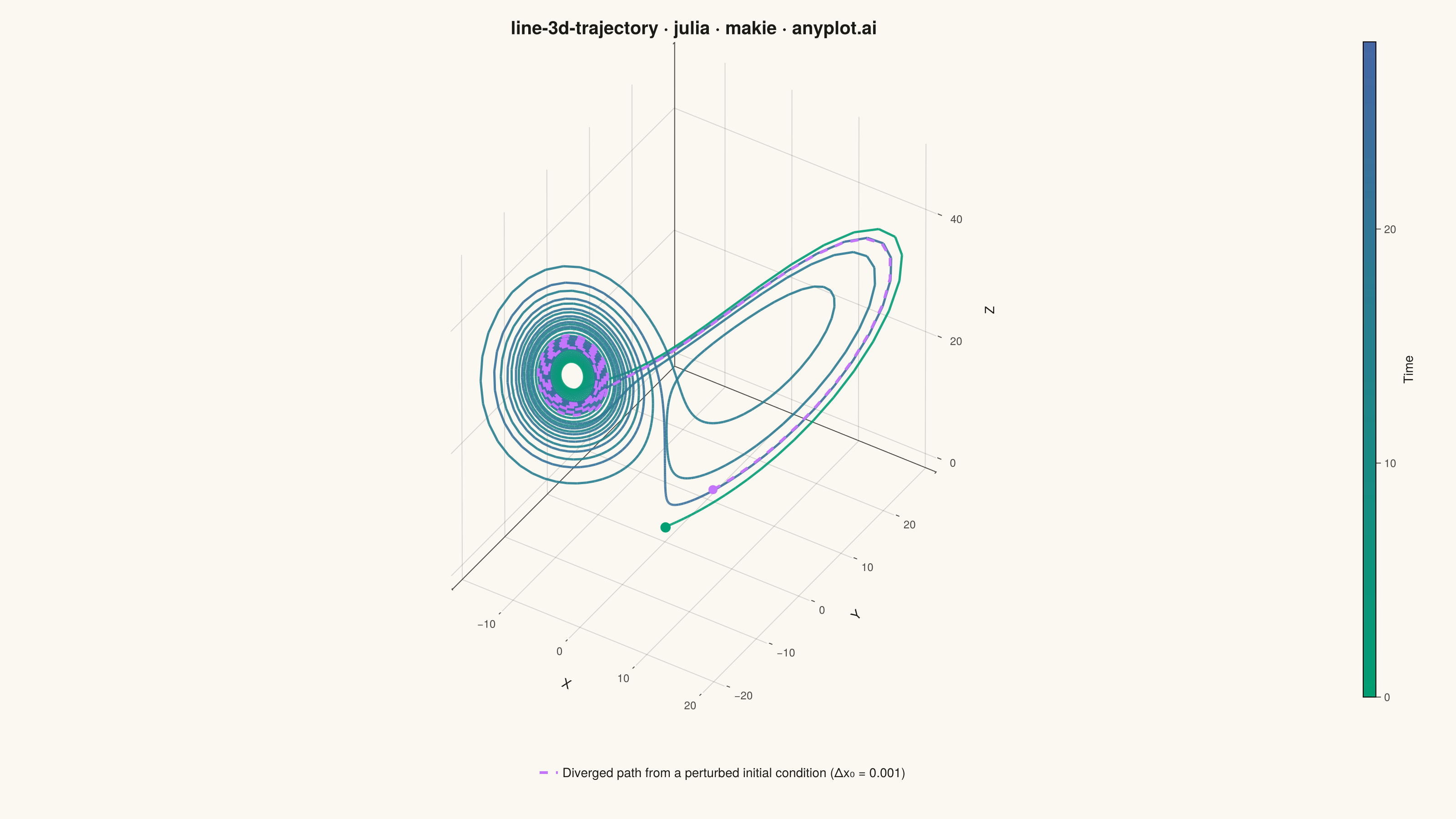
A 3D line plot that displays paths, trajectories, or curves as connected lines in three-dimensional space. Unlike scatter plots that show discrete points, this visualization connects data points sequentially to reveal continuous paths, making it ideal for understanding motion, mathematical curves, and temporal evolution in 3D. Interactive rotation is essential for exploring the spatial structure of complex trajectories.
# anyplot.ai
# line-3d-trajectory: 3D Line Plot for Trajectory Visualization
# Library: makie 0.21.9 | Julia 1.11.9
# Quality: 89/100 | Created: 2026-09-10

using CairoMakie
using Colors

# --- Theme tokens -----------------------------------------------------------
THEME       = get(ENV, "ANYPLOT_THEME", "light")
PAGE_BG     = THEME == "light" ? colorant"#FAF8F1" : colorant"#1A1A17"
ELEVATED_BG = THEME == "light" ? colorant"#FFFDF6" : colorant"#242420"
INK         = THEME == "light" ? colorant"#1A1A17" : colorant"#F0EFE8"
INK_SOFT    = THEME == "light" ? colorant"#4A4A44" : colorant"#B8B7B0"

IMPRINT_PALETTE = [
    colorant"#009E73", colorant"#C475FD", colorant"#4467A3", colorant"#BD8233",
    colorant"#AE3030", colorant"#2ABCCD", colorant"#954477", colorant"#99B314",
]
ANYPLOT_SEQ = cgrad([colorant"#009E73", colorant"#4467A3"])  # sequential — time progression

# --- Data: Lorenz attractor trajectory (classic chaotic system) ------------
sigma, rho, beta = 10.0, 28.0, 8.0 / 3.0
dt = 0.014
n_steps = 2000

function integrate_lorenz(x0, y0, z0, n_steps, dt, sigma, rho, beta)
    xs, ys, zs = zeros(n_steps), zeros(n_steps), zeros(n_steps)
    xs[1], ys[1], zs[1] = x0, y0, z0

    for i in 1:(n_steps - 1)
        xi, yi, zi = xs[i], ys[i], zs[i]

        k1x, k1y, k1z = sigma * (yi - xi), xi * (rho - zi) - yi, xi * yi - beta * zi
        xa, ya, za = xi + 0.5dt * k1x, yi + 0.5dt * k1y, zi + 0.5dt * k1z

        k2x, k2y, k2z = sigma * (ya - xa), xa * (rho - za) - ya, xa * ya - beta * za
        xb, yb, zb = xi + 0.5dt * k2x, yi + 0.5dt * k2y, zi + 0.5dt * k2z

        k3x, k3y, k3z = sigma * (yb - xb), xb * (rho - zb) - yb, xb * yb - beta * zb
        xc, yc, zc = xi + dt * k3x, yi + dt * k3y, zi + dt * k3z

        k4x, k4y, k4z = sigma * (yc - xc), xc * (rho - zc) - yc, xc * yc - beta * zc

        xs[i + 1] = xi + (dt / 6) * (k1x + 2k2x + 2k3x + k4x)
        ys[i + 1] = yi + (dt / 6) * (k1y + 2k2y + 2k3y + k4y)
        zs[i + 1] = zi + (dt / 6) * (k1z + 2k2z + 2k3z + k4z)
    end

    return xs, ys, zs
end

# Two nearby initial conditions illustrate chaotic sensitivity: the paths
# stay close for most of the run, then fork apart once the perturbation has
# grown enough to be visible — the hallmark "butterfly effect" of this system.
traj_x, traj_y, traj_z = integrate_lorenz(0.1, 0.0, 0.0, n_steps, dt, sigma, rho, beta)
traj2_x, traj2_y, traj2_z = integrate_lorenz(0.1 + 1.0e-3, 0.0, 0.0, n_steps, dt, sigma, rho, beta)

separation = sqrt.((traj_x .- traj2_x) .^ 2 .+ (traj_y .- traj2_y) .^ 2 .+ (traj_z .- traj2_z) .^ 2)
fork_idx = something(findfirst(d -> d > 2.0, separation), n_steps ÷ 2)

# --- Plot ---------------------------------------------------------------
fig = Figure(
    size            = (1600, 900),
    fontsize        = 14,
    backgroundcolor = PAGE_BG,
)

ax = Axis3(
    fig[1, 1];
    title              = "line-3d-trajectory · julia · makie · anyplot.ai",
    titlesize          = 20,
    titlecolor         = INK,
    xlabel             = "X",
    ylabel             = "Y",
    zlabel             = "Z",
    xlabelsize         = 14,
    ylabelsize         = 14,
    zlabelsize         = 14,
    xlabelcolor        = INK,
    ylabelcolor        = INK,
    zlabelcolor        = INK,
    xticklabelsize     = 12,
    yticklabelsize     = 12,
    zticklabelsize     = 12,
    xticklabelcolor    = INK_SOFT,
    yticklabelcolor    = INK_SOFT,
    zticklabelcolor    = INK_SOFT,
    xtickcolor         = INK_SOFT,
    ytickcolor         = INK_SOFT,
    ztickcolor         = INK_SOFT,
    xgridcolor         = RGBAf(INK.r, INK.g, INK.b, 0.15),
    ygridcolor         = RGBAf(INK.r, INK.g, INK.b, 0.15),
    zgridcolor         = RGBAf(INK.r, INK.g, INK.b, 0.15),
    xspinecolor_1      = INK_SOFT,
    yspinecolor_1      = INK_SOFT,
    zspinecolor_1      = INK_SOFT,
    xspinecolor_2      = INK_SOFT,
    yspinecolor_2      = INK_SOFT,
    zspinecolor_2      = INK_SOFT,
    xspinecolor_3      = INK_SOFT,
    yspinecolor_3      = INK_SOFT,
    zspinecolor_3      = INK_SOFT,
    xypanelcolor       = PAGE_BG,
    yzpanelcolor       = PAGE_BG,
    xzpanelcolor       = PAGE_BG,
    backgroundcolor    = PAGE_BG,
    aspect             = :data,
    elevation          = 0.22 * pi,
    azimuth            = -0.32 * pi,
)

lines!(ax, traj_x, traj_y, traj_z; color = 1:n_steps, colormap = ANYPLOT_SEQ, linewidth = 2.5, alpha = 0.9)
scatter!(ax, [traj_x[1]], [traj_y[1]], [traj_z[1]]; color = IMPRINT_PALETTE[1], markersize = 16, strokewidth = 0)

# The perturbed run shares the same path as the main trajectory up to
# `fork_idx`; only the diverged tail is drawn, so the fork itself is the
# visible story rather than two fully overlapping lines. A dashed style
# (on top of the distinct lavender color) keeps the diverged path readable
# even where it briefly re-overlaps the main spiral.
traj2_line = lines!(
    ax, traj2_x[fork_idx:end], traj2_y[fork_idx:end], traj2_z[fork_idx:end];
    color = IMPRINT_PALETTE[2], linewidth = 3.0, linestyle = :dash, alpha = 1.0,
)
scatter!(ax, [traj2_x[fork_idx]], [traj2_y[fork_idx]], [traj2_z[fork_idx]]; color = IMPRINT_PALETTE[2], markersize = 14, strokewidth = 0)

Colorbar(
    fig[1, 2];
    limits       = (0, n_steps * dt),
    colormap     = ANYPLOT_SEQ,
    label        = "Time",
    labelsize    = 14,
    labelcolor   = INK,
    ticklabelsize = 12,
    ticklabelcolor = INK_SOFT,
    tickcolor    = INK_SOFT,
    width        = 14,
)

Legend(
    fig[2, 1:2],
    [traj2_line],
    ["Diverged path from a perturbed initial condition (Δx₀ = 0.001)"];
    orientation     = :horizontal,
    framevisible    = false,
    backgroundcolor = :transparent,
    labelcolor      = INK,
    tellwidth       = false,
    tellheight      = true,
)

colsize!(fig.layout, 1, Relative(0.95))
rowsize!(fig.layout, 1, Auto(1.0))
rowsize!(fig.layout, 2, Fixed(70))

# --- Save -----------------------------------------------------------------
save("plot-$(THEME).png", fig; px_per_unit = 2)
Runnable source as JSON, for any HTTP client: https://api.anyplot.ai/specs/line-3d-trajectory/makie/code. Any spec id and library id listed in llms-full.txt fit the same URL shape; every URL below is complete and callable.
{
  "spec_id": "line-3d-trajectory",
  "language": "julia",
  "library": "makie",
  "page": "https://anyplot.ai/line-3d-trajectory/julia/makie",
  "hub": "https://anyplot.ai/line-3d-trajectory",
  "code_json": "https://api.anyplot.ai/specs/line-3d-trajectory/makie/code",
  "spec_json": "https://api.anyplot.ai/specs/line-3d-trajectory",
  "render_light_png": "https://storage.googleapis.com/anyplot-images/plots/line-3d-trajectory/julia/makie/plot-light.png",
  "render_dark_png": "https://storage.googleapis.com/anyplot-images/plots/line-3d-trajectory/julia/makie/plot-dark.png",
  "quality_score": 89.0,
  "license": "MIT",
  "guide": "https://anyplot.ai/llms.txt"
}
Part of 3D Line Plot for Trajectory Visualization on anyplot.ai.