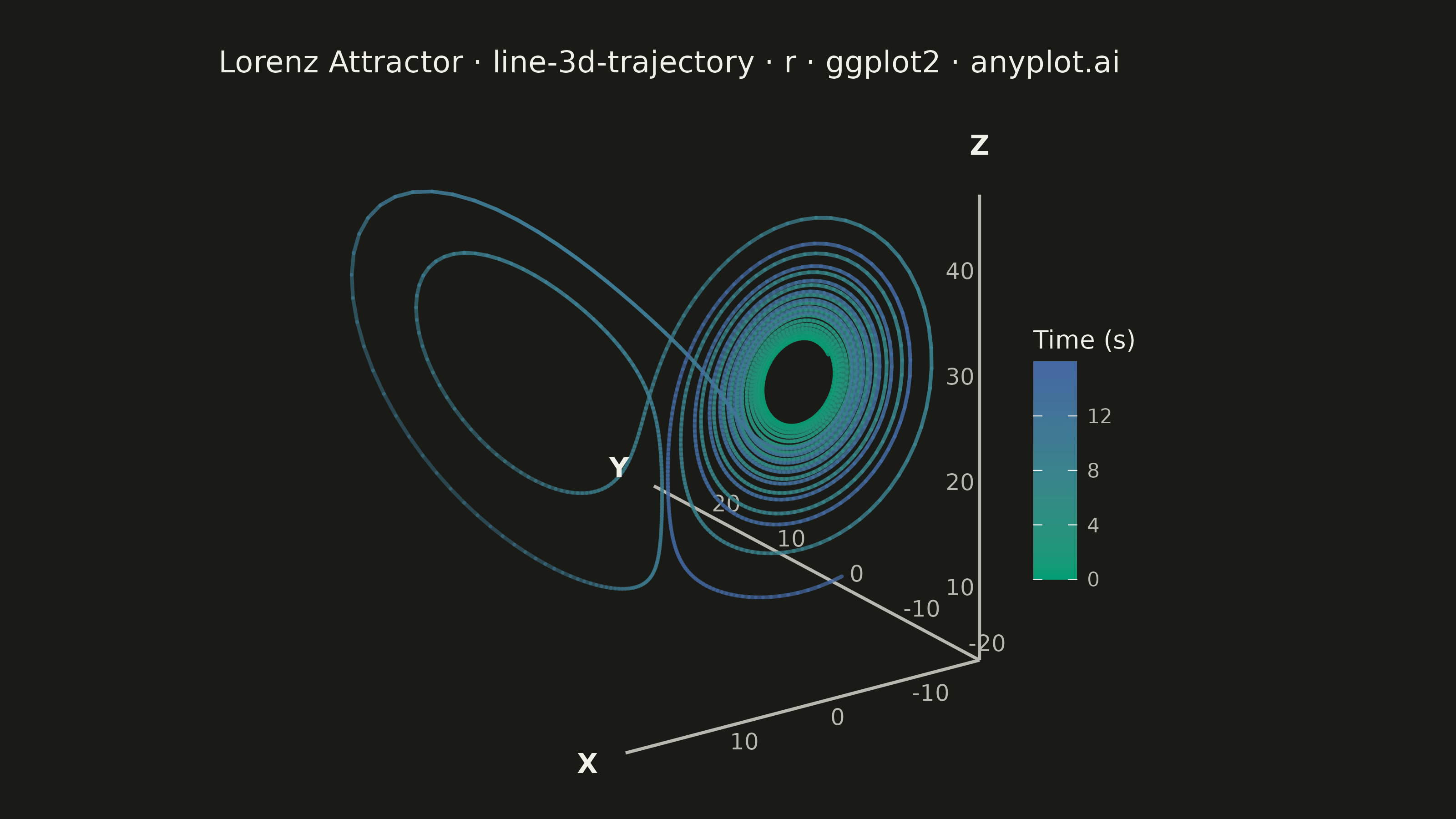
The same plot in 13 other libraries — Python: Altair, Bokeh, lets-plot, Matplotlib, Plotly, Pygal, Seaborn; Julia: Makie.jl; JavaScript: Chart.js, D3.js, Apache ECharts, Highcharts, MUI X Charts. Compare all 14 side by side: 3D Line Plot for Trajectory Visualization in Python, R, Julia and JavaScript.
A 3D line plot that displays paths, trajectories, or curves as connected lines in three-dimensional space. Unlike scatter plots that show discrete points, this visualization connects data points sequentially to reveal continuous paths, making it ideal for understanding motion, mathematical curves, and temporal evolution in 3D. Interactive rotation is essential for exploring the spatial structure of complex trajectories.
#' anyplot.ai
#' line-3d-trajectory: 3D Line Plot for Trajectory Visualization
#' Library: ggplot2 3.5.1 | R 4.4.1
#' Quality: 87/100 | Created: 2026-09-10

library(ggplot2)
library(ragg)

set.seed(42)

# --- Theme tokens -------------------------------------------------------------
THEME    <- Sys.getenv("ANYPLOT_THEME", "light")
PAGE_BG  <- if (THEME == "light") "#FAF8F1" else "#1A1A17"
INK      <- if (THEME == "light") "#1A1A17" else "#F0EFE8"
INK_SOFT <- if (THEME == "light") "#4A4A44" else "#B8B7B0"

# --- Camera: orthographic projection (elevation 22, azimuth -55) --------------
# ggplot2 has no 3D grammar, so the trajectory is projected to 2D screen
# coordinates ourselves (the same technique any static 3D renderer uses under
# the hood), then drawn with plain geom_path/geom_segment/geom_text.
elev <- 22 * pi / 180
azim <- -55 * pi / 180

view_dir   <- c(cos(elev) * cos(azim), cos(elev) * sin(azim), sin(elev))
world_up   <- c(0, 0, 1)
right_axis <- c(
  view_dir[2] * world_up[3] - view_dir[3] * world_up[2],
  view_dir[3] * world_up[1] - view_dir[1] * world_up[3],
  view_dir[1] * world_up[2] - view_dir[2] * world_up[1]
)
right_axis <- right_axis / sqrt(sum(right_axis^2))
up_axis <- c(
  right_axis[2] * view_dir[3] - right_axis[3] * view_dir[2],
  right_axis[3] * view_dir[1] - right_axis[1] * view_dir[3],
  right_axis[1] * view_dir[2] - right_axis[2] * view_dir[1]
)

project_x <- function(x, y, z) x * right_axis[1] + y * right_axis[2] + z * right_axis[3]
project_y <- function(x, y, z) x * up_axis[1]    + y * up_axis[2]    + z * up_axis[3]
depth_of  <- function(x, y, z) x * view_dir[1]   + y * view_dir[2]   + z * view_dir[3]

# --- Data: Lorenz attractor, integrated with classic RK4 -----------------------
sigma <- 10
rho   <- 28
beta  <- 8 / 3
dt    <- 0.008
n_burn  <- 1000   # discard the transient before the state settles onto the attractor
n_steps <- 2000

lorenz_rhs <- function(s) {
  c(
    sigma * (s[2] - s[1]),
    s[1] * (rho - s[3]) - s[2],
    s[1] * s[2] - beta * s[3]
  )
}

rk4_step <- function(s, dt) {
  k1 <- lorenz_rhs(s)
  k2 <- lorenz_rhs(s + dt / 2 * k1)
  k3 <- lorenz_rhs(s + dt / 2 * k2)
  k4 <- lorenz_rhs(s + dt * k3)
  s + dt / 6 * (k1 + 2 * k2 + 2 * k3 + k4)
}

state <- c(x = 0.1, y = 0, z = 0)
for (i in seq_len(n_burn)) state <- rk4_step(state, dt)

traj <- matrix(NA_real_, nrow = n_steps, ncol = 3, dimnames = list(NULL, c("x", "y", "z")))
for (i in seq_len(n_steps)) {
  state <- rk4_step(state, dt)
  traj[i, ] <- state
}
traj <- as.data.frame(traj)
traj$t <- (seq_len(n_steps) - 1) * dt

traj$px         <- project_x(traj$x, traj$y, traj$z)
traj$py         <- project_y(traj$x, traj$y, traj$z)
traj$depth      <- depth_of(traj$x, traj$y, traj$z)
depth_rng       <- range(traj$depth)
traj$depth_norm <- (traj$depth - depth_rng[1]) / diff(depth_rng)

# --- Axis box: three edges meeting at the near-bottom corner -------------------
xr <- range(traj$x)
yr <- range(traj$y)
zr <- range(traj$z)
x_pad <- diff(xr) * 0.06
y_pad <- diff(yr) * 0.06
z_pad <- diff(zr) * 0.06

corner <- c(xr[1] - x_pad, yr[1] - y_pad, zr[1] - z_pad)

axis_lines <- data.frame(
  x    = rep(corner[1], 3),
  y    = rep(corner[2], 3),
  z    = rep(corner[3], 3),
  xend = c(xr[2] + x_pad, corner[1], corner[1]),
  yend = c(corner[2], yr[2] + y_pad, corner[2]),
  zend = c(corner[3], corner[3], zr[2] + z_pad)
)
axis_lines$px    <- project_x(axis_lines$x, axis_lines$y, axis_lines$z)
axis_lines$py    <- project_y(axis_lines$x, axis_lines$y, axis_lines$z)
axis_lines$pxend <- project_x(axis_lines$xend, axis_lines$yend, axis_lines$zend)
axis_lines$pyend <- project_y(axis_lines$xend, axis_lines$yend, axis_lines$zend)

x_breaks <- pretty(xr, n = 4)
x_breaks <- x_breaks[x_breaks >= xr[1] & x_breaks <= xr[2]]
y_breaks <- pretty(yr, n = 4)
y_breaks <- y_breaks[y_breaks >= yr[1] & y_breaks <= yr[2]]
z_breaks <- pretty(zr, n = 4)
z_breaks <- z_breaks[z_breaks >= zr[1] & z_breaks <= zr[2]]

x_ticks <- data.frame(x = x_breaks, y = corner[2] - y_pad * 1.4, z = corner[3], label = x_breaks)
y_ticks <- data.frame(x = corner[1] - x_pad * 1.4, y = y_breaks, z = corner[3], label = y_breaks)
x_ticks$px <- project_x(x_ticks$x, x_ticks$y, x_ticks$z)
x_ticks$py <- project_y(x_ticks$x, x_ticks$y, x_ticks$z)
y_ticks$px <- project_x(y_ticks$x, y_ticks$y, y_ticks$z)
y_ticks$py <- project_y(y_ticks$x, y_ticks$y, y_ticks$z)

# Z ticks sit on the vertical axis line; nudge the label sideways in pixel
# space so it doesn't merge with the axis line itself.
z_ticks <- data.frame(x = corner[1], y = corner[2], z = z_breaks, label = z_breaks)
z_ticks$px <- project_x(z_ticks$x, z_ticks$y, z_ticks$z) - diff(xr) * 0.05
z_ticks$py <- project_y(z_ticks$x, z_ticks$y, z_ticks$z)

axis_labels <- data.frame(
  x     = c(xr[2] + x_pad * 3, corner[1], corner[1]),
  y     = c(corner[2], yr[2] + y_pad * 3, corner[2]),
  z     = c(corner[3], corner[3], zr[2] + z_pad * 3),
  label = c("X", "Y", "Z")
)
axis_labels$px <- project_x(axis_labels$x, axis_labels$y, axis_labels$z)
axis_labels$py <- project_y(axis_labels$x, axis_labels$y, axis_labels$z)

# --- Plot -----------------------------------------------------------------
p <- ggplot() +
  geom_segment(data = axis_lines, aes(x = px, y = py, xend = pxend, yend = pyend),
               color = INK_SOFT, linewidth = 0.6) +
  geom_text(data = x_ticks, aes(px, py, label = label), color = INK_SOFT, size = 3.2) +
  geom_text(data = y_ticks, aes(px, py, label = label), color = INK_SOFT, size = 3.2) +
  geom_text(data = z_ticks, aes(px, py, label = label), color = INK_SOFT, size = 3.2) +
  geom_path(data = traj, aes(px, py, color = t, alpha = depth_norm),
            linewidth = 0.7, lineend = "round") +
  geom_text(data = axis_labels, aes(px, py, label = label),
            color = INK, size = 3.8, fontface = "bold") +
  scale_color_gradient(low = "#009E73", high = "#4467A3", name = "Time (s)") +
  scale_alpha_continuous(range = c(0.45, 1), guide = "none") +
  labs(title = "Lorenz Attractor · line-3d-trajectory · r · ggplot2 · anyplot.ai") +
  coord_fixed(ratio = 1, clip = "off") +
  theme_void(base_size = 8) +
  theme(
    plot.background  = element_rect(fill = PAGE_BG, color = PAGE_BG),
    panel.background = element_rect(fill = PAGE_BG, color = NA),
    plot.title       = element_text(color = INK, size = 12, hjust = 0.5, margin = margin(b = 14)),
    legend.position  = "right",
    legend.title     = element_text(color = INK, size = 10),
    legend.text      = element_text(color = INK_SOFT, size = 8),
    legend.key       = element_rect(fill = PAGE_BG, color = NA),
    plot.margin      = margin(t = 20, r = 20, b = 10, l = 20)
  )

# --- Save -----------------------------------------------------------------
ggsave(
  filename = sprintf("plot-%s.png", THEME),
  plot     = p,
  device   = ragg::agg_png,
  width    = 8,
  height   = 4.5,
  units    = "in",
  dpi      = 400
)
Runnable source as JSON, for any HTTP client: https://api.anyplot.ai/specs/line-3d-trajectory/ggplot2/code. Any spec id and library id listed in llms-full.txt fit the same URL shape; every URL below is complete and callable.
{
  "spec_id": "line-3d-trajectory",
  "language": "r",
  "library": "ggplot2",
  "page": "https://anyplot.ai/line-3d-trajectory/r/ggplot2",
  "hub": "https://anyplot.ai/line-3d-trajectory",
  "code_json": "https://api.anyplot.ai/specs/line-3d-trajectory/ggplot2/code",
  "spec_json": "https://api.anyplot.ai/specs/line-3d-trajectory",
  "render_light_png": "https://storage.googleapis.com/anyplot-images/plots/line-3d-trajectory/r/ggplot2/plot-light.png",
  "render_dark_png": "https://storage.googleapis.com/anyplot-images/plots/line-3d-trajectory/r/ggplot2/plot-dark.png",
  "quality_score": 87.0,
  "license": "MIT",
  "guide": "https://anyplot.ai/llms.txt"
}
Part of 3D Line Plot for Trajectory Visualization on anyplot.ai.