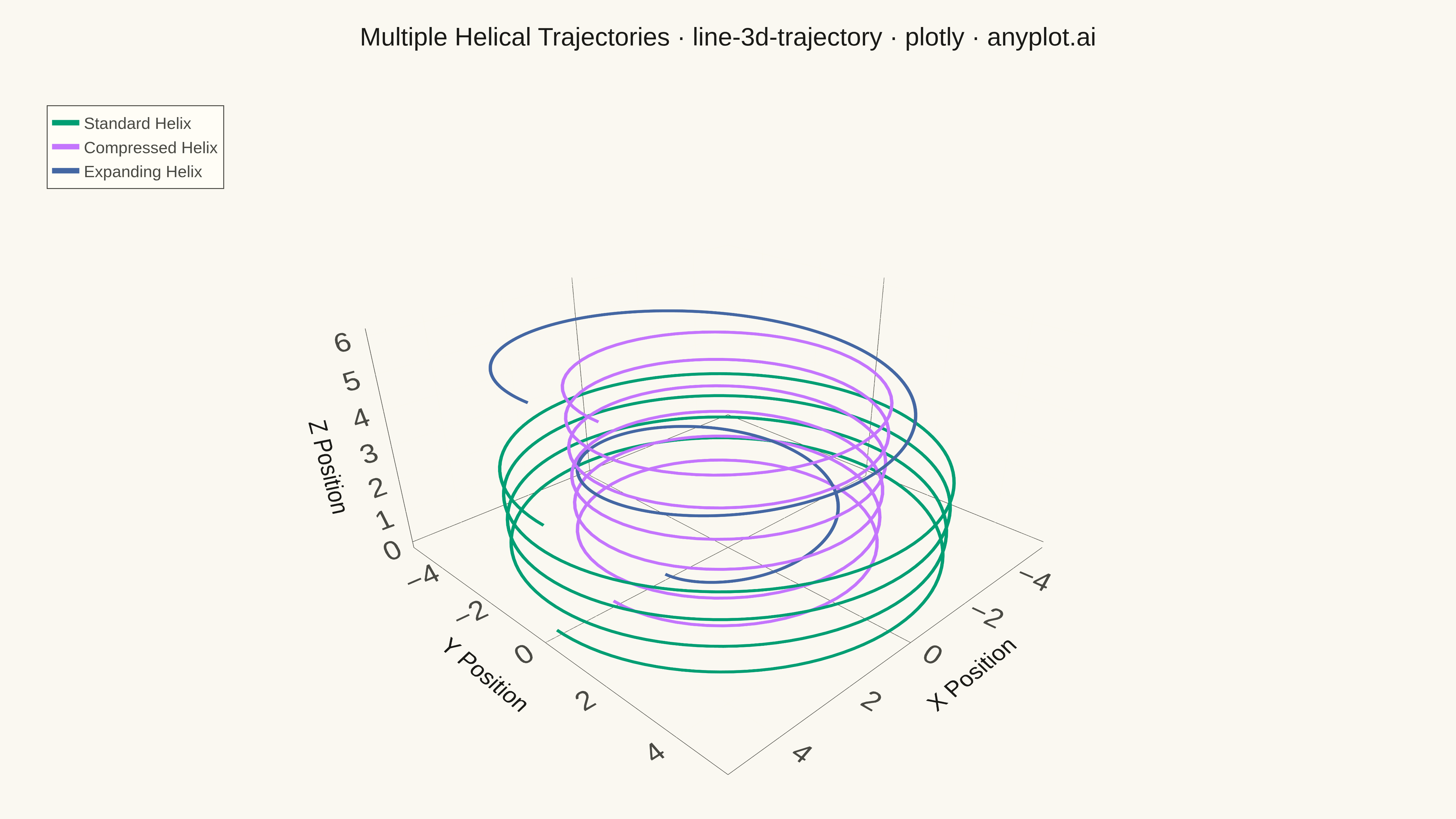
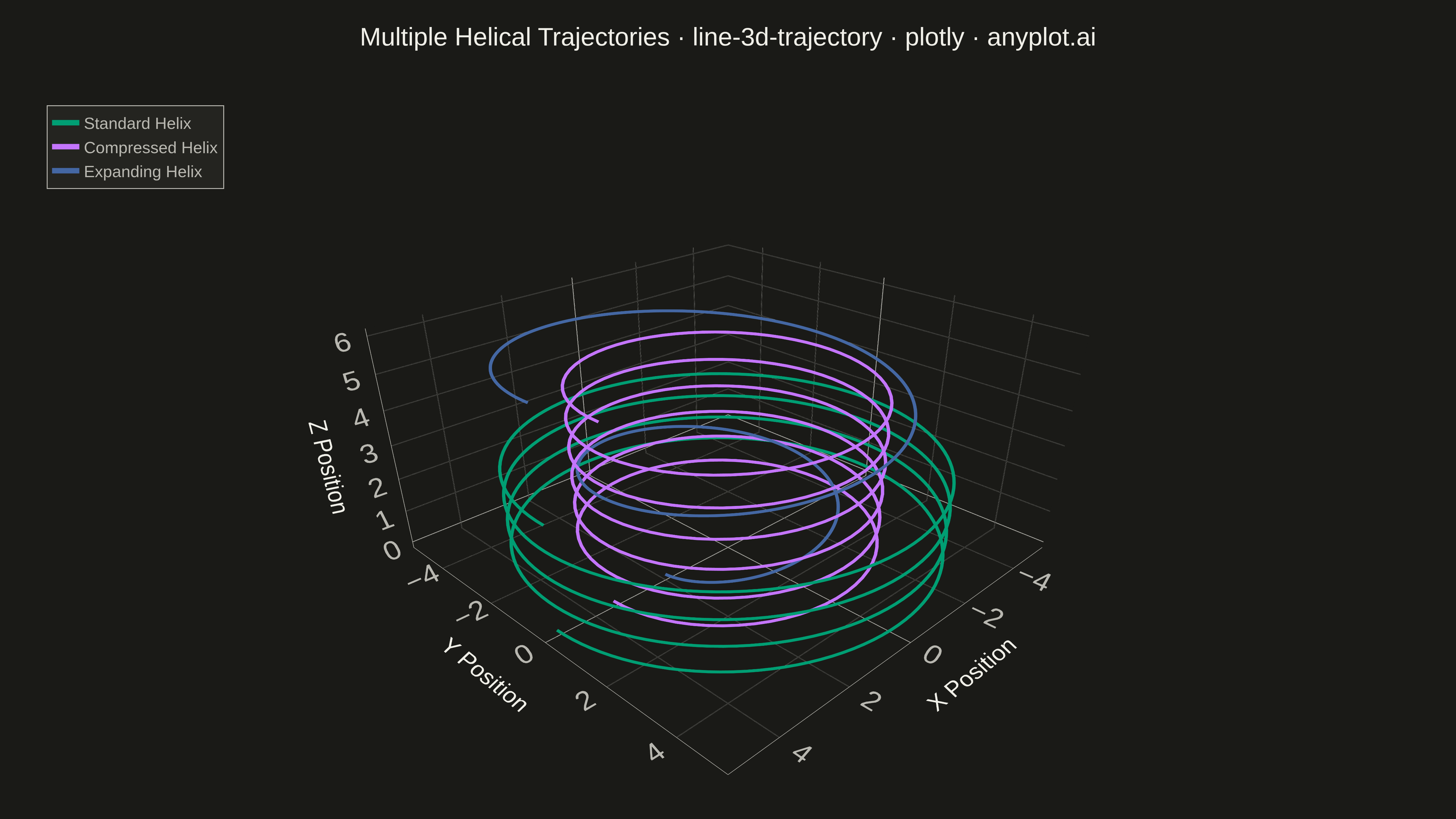
A 3D line plot that displays paths, trajectories, or curves as connected lines in three-dimensional space. Unlike scatter plots that show discrete points, this visualization connects data points sequentially to reveal continuous paths, making it ideal for understanding motion, mathematical curves, and temporal evolution in 3D. Interactive rotation is essential for exploring the spatial structure of complex trajectories.
""" anyplot.ai
line-3d-trajectory: 3D Line Plot for Trajectory Visualization
Library: plotly 6.7.0 | Python 3.13.13
Quality: 96/100 | Updated: 2026-05-16
"""

import os
import sys

import numpy as np


# Avoid shadowing plotly package when script is named plotly.py
while sys.path and (sys.path[0] == "" or sys.path[0].endswith("/python")):
    sys.path.pop(0)

import plotly.graph_objects as go


# Theme tokens (see prompts/default-style-guide.md "Background" + "Theme-adaptive Chrome")
THEME = os.getenv("ANYPLOT_THEME", "light")
PAGE_BG = "#FAF8F1" if THEME == "light" else "#1A1A17"
ELEVATED_BG = "#FFFDF6" if THEME == "light" else "#242420"
INK = "#1A1A17" if THEME == "light" else "#F0EFE8"
INK_SOFT = "#4A4A44" if THEME == "light" else "#B8B7B0"
GRID = "rgba(26,26,23,0.10)" if THEME == "light" else "rgba(240,239,232,0.10)"

IMPRINT = ["#009E73", "#C475FD", "#4467A3", "#BD8233", "#AE3030", "#2ABCCD"]

# Data: Multiple 3D helix trajectories with different periods and amplitudes
np.random.seed(42)

# Parameters for three helical trajectories
trajectories = []
labels = []

# Helix 1: Standard helix
t1 = np.linspace(0, 8 * np.pi, 500)
x1 = 5 * np.cos(t1)
y1 = 5 * np.sin(t1)
z1 = 3 * t1 / (8 * np.pi)
trajectories.append((x1, y1, z1, IMPRINT[0]))
labels.append("Standard Helix")

# Helix 2: Compressed helix (faster rise, tighter spiral)
t2 = np.linspace(0, 6 * np.pi, 400)
x2 = 3.5 * np.cos(2 * t2)
y2 = 3.5 * np.sin(2 * t2)
z2 = 5 * t2 / (6 * np.pi)
trajectories.append((x2, y2, z2, IMPRINT[1]))
labels.append("Compressed Helix")

# Helix 3: Expanding helix (amplitude increases with height)
t3 = np.linspace(0, 4 * np.pi, 400)
amplitude = 2 + 3 * (t3 / (4 * np.pi))
x3 = amplitude * np.cos(t3)
y3 = amplitude * np.sin(t3)
z3 = 6 * t3 / (4 * np.pi)
trajectories.append((x3, y3, z3, IMPRINT[2]))
labels.append("Expanding Helix")

# Create 3D line plot with multiple trajectories
fig = go.Figure()

for (x, y, z, color), label in zip(trajectories, labels, strict=True):
    fig.add_trace(
        go.Scatter3d(
            x=x,
            y=y,
            z=z,
            mode="lines",
            name=label,
            line=dict(color=color, width=6),
            hovertemplate=f"{label}<br>X: %{{x:.2f}}<br>Y: %{{y:.2f}}<br>Z: %{{z:.2f}}<extra></extra>",
        )
    )

# Update layout for 4800x2700 output
fig.update_layout(
    title=dict(
        text="Multiple Helical Trajectories · line-3d-trajectory · plotly · anyplot.ai",
        font=dict(size=28, color=INK),
        x=0.5,
        xanchor="center",
    ),
    scene=dict(
        xaxis=dict(
            title=dict(text="X Position", font=dict(size=22, color=INK)),
            tickfont=dict(size=18, color=INK_SOFT),
            gridcolor=GRID,
            showbackground=True,
            backgroundcolor=PAGE_BG,
            linecolor=INK_SOFT,
            zerolinecolor=INK_SOFT,
        ),
        yaxis=dict(
            title=dict(text="Y Position", font=dict(size=22, color=INK)),
            tickfont=dict(size=18, color=INK_SOFT),
            gridcolor=GRID,
            showbackground=True,
            backgroundcolor=PAGE_BG,
            linecolor=INK_SOFT,
            zerolinecolor=INK_SOFT,
        ),
        zaxis=dict(
            title=dict(text="Z Position", font=dict(size=22, color=INK)),
            tickfont=dict(size=18, color=INK_SOFT),
            gridcolor=GRID,
            showbackground=True,
            backgroundcolor=PAGE_BG,
            linecolor=INK_SOFT,
            zerolinecolor=INK_SOFT,
        ),
        camera=dict(eye=dict(x=1.5, y=1.5, z=1.2)),
        aspectmode="data",
    ),
    paper_bgcolor=PAGE_BG,
    plot_bgcolor=PAGE_BG,
    font=dict(color=INK),
    legend=dict(
        x=0.02, y=0.98, bgcolor=ELEVATED_BG, bordercolor=INK_SOFT, borderwidth=1, font=dict(size=18, color=INK_SOFT)
    ),
    margin=dict(l=20, r=20, t=100, b=20),
    hovermode="closest",
)

# Save as PNG (4800x2700) and HTML
fig.write_image(f"plot-{THEME}.png", width=1600, height=900, scale=3)
fig.write_html(f"plot-{THEME}.html", include_plotlyjs="cdn")
Runnable source as JSON, for any HTTP client: https://api.anyplot.ai/specs/line-3d-trajectory/plotly/code. Any spec id and library id listed in llms-full.txt fit the same URL shape; every URL below is complete and callable.
{
  "spec_id": "line-3d-trajectory",
  "language": "python",
  "library": "plotly",
  "page": "https://anyplot.ai/line-3d-trajectory/python/plotly",
  "hub": "https://anyplot.ai/line-3d-trajectory",
  "code_json": "https://api.anyplot.ai/specs/line-3d-trajectory/plotly/code",
  "spec_json": "https://api.anyplot.ai/specs/line-3d-trajectory",
  "render_light_png": "https://storage.googleapis.com/anyplot-images/plots/line-3d-trajectory/python/plotly/plot-light.png",
  "render_dark_png": "https://storage.googleapis.com/anyplot-images/plots/line-3d-trajectory/python/plotly/plot-dark.png",
  "interactive_light_html": "https://storage.googleapis.com/anyplot-images/plots/line-3d-trajectory/python/plotly/plot-light.html",
  "interactive_dark_html": "https://storage.googleapis.com/anyplot-images/plots/line-3d-trajectory/python/plotly/plot-dark.html",
  "quality_score": 96.0,
  "license": "MIT",
  "guide": "https://anyplot.ai/llms.txt"
}
Part of 3D Line Plot for Trajectory Visualization on anyplot.ai.