The same plot in 14 other libraries — JavaScript: D3.js, Apache ECharts, Highcharts, MUI X Charts; Python: Altair, Bokeh, lets-plot, Matplotlib, Plotly, plotnine, Pygal, Seaborn; R: ggplot2; Julia: Makie.jl. Compare all 15 side by side: Arrhenius Plot for Reaction Kinetics in Python, R, Julia and JavaScript.
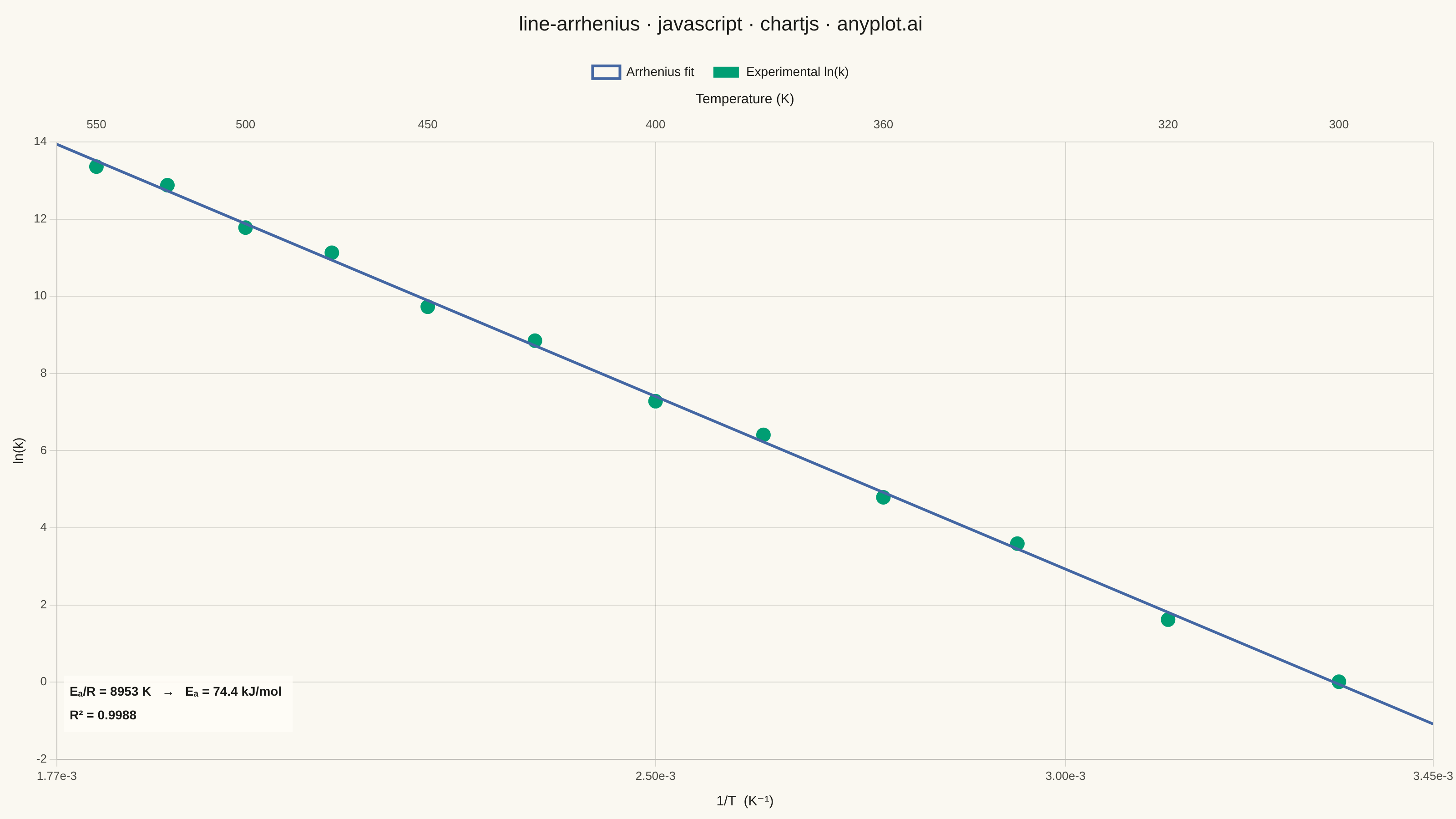
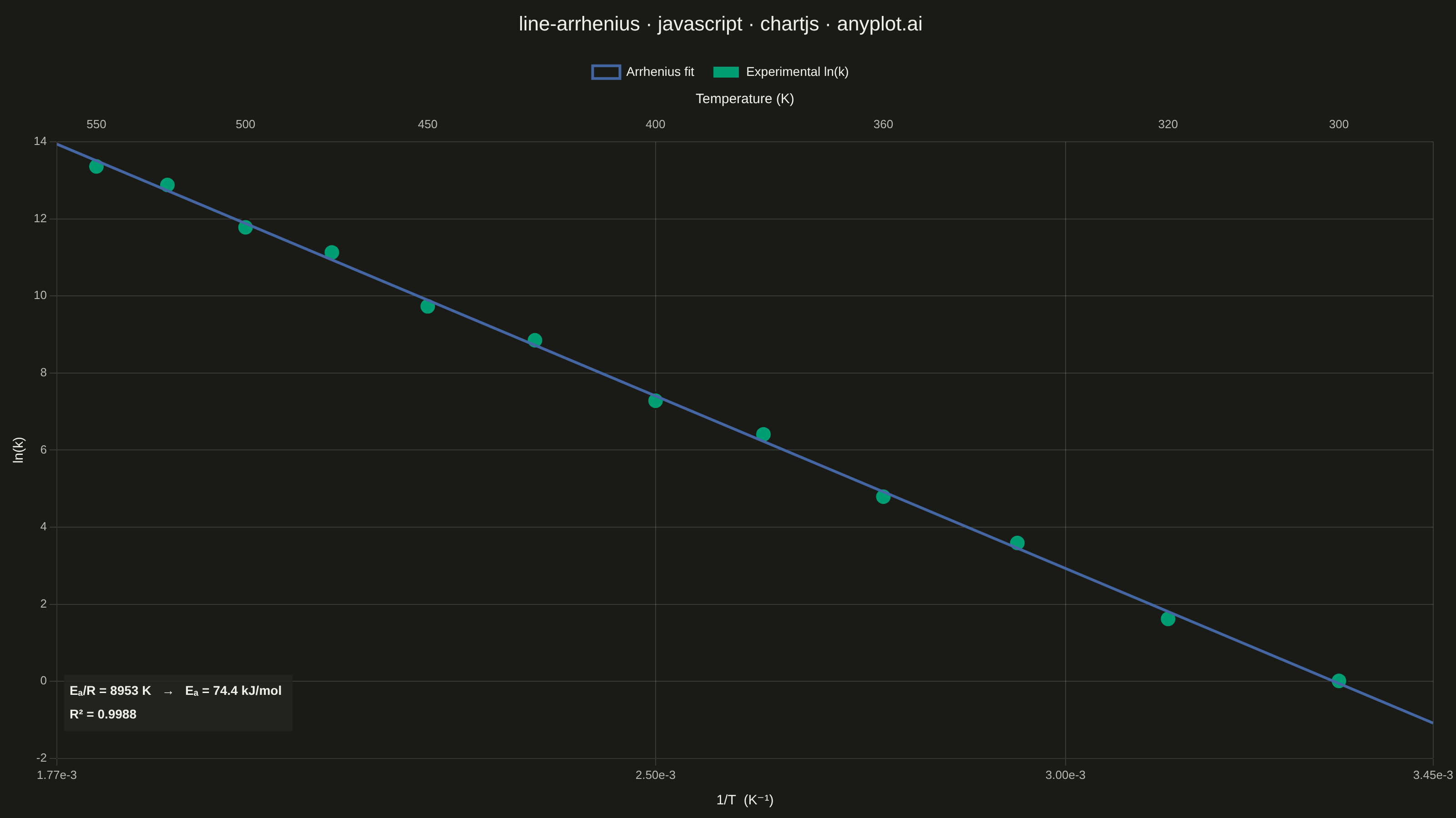
An Arrhenius plot displays ln(k) versus 1/T to determine the activation energy of a chemical reaction from experimental rate constant data. The Arrhenius equation predicts a linear relationship on this transformed scale, where the slope equals -Ea/R (activation energy divided by the gas constant). This visualization is fundamental in physical chemistry and chemical engineering for characterizing reaction kinetics and comparing catalytic performance.
// anyplot.ai
// line-arrhenius: Arrhenius Plot for Reaction Kinetics
// Library: chartjs 4.4.7 | JavaScript 22.22.3
// Quality: 91/100 | Created: 2026-06-24

const t = window.ANYPLOT_TOKENS;

// H₂O₂ decomposition over MnO₂ catalyst — experimental ln(k) vs 1/T
const temperatures = [300, 320, 340, 360, 380, 400, 425, 450, 475, 500, 525, 550];
const lnK = [0.01, 1.62, 3.59, 4.79, 6.41, 7.28, 8.85, 9.73, 11.13, 11.78, 12.88, 13.36];
const invT = temperatures.map(T => 1 / T);

// Linear regression: slope = -Ea/R, intercept = ln(A)
const nn = invT.length;
const xm = invT.reduce((a, b) => a + b, 0) / nn;
const ym = lnK.reduce((a, b) => a + b, 0) / nn;
const slope = invT.reduce((s, x, i) => s + (x - xm) * (lnK[i] - ym), 0) /
              invT.reduce((s, x) => s + (x - xm) ** 2, 0);
const intercept = ym - slope * xm;

// R² and activation energy
const ssTot = lnK.reduce((s, y) => s + (y - ym) ** 2, 0);
const ssRes = invT.reduce((s, x, i) => s + (lnK[i] - (slope * x + intercept)) ** 2, 0);
const r2 = 1 - ssRes / ssTot;
const Ea_kJ = (-slope * 8.314 / 1000).toFixed(1);

// x-axis bounds (slightly wider than data range)
const X_MIN = 1 / 565;
const X_MAX = 1 / 290;

const scatterData = invT.map((x, i) => ({ x, y: lnK[i] }));
const regLineData = [
    { x: X_MIN, y: slope * X_MIN + intercept },
    { x: X_MAX, y: slope * X_MAX + intercept },
];

const canvas = document.createElement("canvas");
document.getElementById("container").appendChild(canvas);

// Inline annotation plugin: Ea/R and R² in bottom-left (away from data cluster)
const annotPlugin = {
    id: "annot",
    afterDraw(chart) {
        const { ctx, chartArea: ca } = chart;
        const line1 = `Eₐ/R = ${(-slope).toFixed(0)} K   →   Eₐ = ${Ea_kJ} kJ/mol`;
        const line2 = `R² = ${r2.toFixed(4)}`;
        const x = ca.left + 14;
        const y1 = ca.bottom - 74;
        const y2 = ca.bottom - 48;
        ctx.save();
        ctx.font = "bold 14px sans-serif";
        const boxW = Math.max(ctx.measureText(line1).width, ctx.measureText(line2).width) + 18;
        ctx.globalAlpha = 0.82;
        ctx.fillStyle = t.elevatedBg;
        ctx.fillRect(x - 6, y1 - 18, boxW, 62);
        ctx.globalAlpha = 1;
        ctx.fillStyle = t.ink;
        ctx.textAlign = "left";
        ctx.fillText(line1, x, y1);
        ctx.fillText(line2, x, y2);
        ctx.restore();
    },
};

const titleStr = "line-arrhenius · javascript · chartjs · anyplot.ai";

new Chart(canvas, {
    data: {
        datasets: [
            {
                type: "line",
                label: "Arrhenius fit",
                data: regLineData,
                borderColor: t.palette[2],
                borderWidth: 3.0,
                backgroundColor: "transparent",
                pointRadius: 0,
                tension: 0,
                fill: false,
            },
            {
                type: "scatter",
                label: "Experimental ln(k)",
                data: scatterData,
                backgroundColor: t.palette[0],
                borderColor: t.pageBg,
                borderWidth: 2,
                pointRadius: 9,
                pointHoverRadius: 11,
            },
        ],
    },
    options: {
        responsive: true,
        maintainAspectRatio: false,
        animation: false,
        layout: { padding: { top: 6, right: 24, bottom: 6, left: 8 } },
        plugins: {
            title: {
                display: true,
                text: titleStr,
                color: t.ink,
                font: { size: 22, weight: "500" },
                padding: { top: 8, bottom: 12 },
            },
            legend: {
                labels: {
                    color: t.ink,
                    font: { size: 14 },
                    padding: 20,
                    boxWidth: 30,
                },
            },
        },
        scales: {
            x: {
                type: "linear",
                min: X_MIN,
                max: X_MAX,
                title: {
                    display: true,
                    text: "1/T  (K⁻¹)",
                    color: t.ink,
                    font: { size: 15 },
                    padding: { top: 8 },
                },
                ticks: {
                    color: t.inkSoft,
                    font: { size: 13 },
                    maxTicksLimit: 8,
                    callback: (v) => v.toExponential(2),
                },
                grid: { color: t.grid },
            },
            y: {
                title: {
                    display: true,
                    text: "ln(k)",
                    color: t.ink,
                    font: { size: 15 },
                },
                ticks: {
                    color: t.inkSoft,
                    font: { size: 13 },
                },
                grid: { color: t.grid },
            },
            x2: {
                type: "linear",
                position: "top",
                min: X_MIN,
                max: X_MAX,
                title: {
                    display: true,
                    text: "Temperature (K)",
                    color: t.ink,
                    font: { size: 15 },
                    padding: { bottom: 8 },
                },
                afterBuildTicks(scale) {
                    scale.ticks = [550, 500, 450, 400, 360, 320, 300].map(T => ({ value: 1 / T }));
                },
                ticks: {
                    color: t.inkSoft,
                    font: { size: 13 },
                    callback: (v) => `${Math.round(1 / v)}`,
                },
                grid: { display: false },
                border: { display: false },
            },
        },
    },
    plugins: [annotPlugin],
});
Runnable source as JSON, for any HTTP client: https://api.anyplot.ai/specs/line-arrhenius/chartjs/code. Any spec id and library id listed in llms-full.txt fit the same URL shape; every URL below is complete and callable.
{
  "spec_id": "line-arrhenius",
  "language": "javascript",
  "library": "chartjs",
  "page": "https://anyplot.ai/line-arrhenius/javascript/chartjs",
  "hub": "https://anyplot.ai/line-arrhenius",
  "code_json": "https://api.anyplot.ai/specs/line-arrhenius/chartjs/code",
  "spec_json": "https://api.anyplot.ai/specs/line-arrhenius",
  "render_light_png": "https://storage.googleapis.com/anyplot-images/plots/line-arrhenius/javascript/chartjs/plot-light.png",
  "render_dark_png": "https://storage.googleapis.com/anyplot-images/plots/line-arrhenius/javascript/chartjs/plot-dark.png",
  "interactive_light_html": "https://storage.googleapis.com/anyplot-images/plots/line-arrhenius/javascript/chartjs/plot-light.html",
  "interactive_dark_html": "https://storage.googleapis.com/anyplot-images/plots/line-arrhenius/javascript/chartjs/plot-dark.html",
  "quality_score": 91.0,
  "license": "MIT",
  "guide": "https://anyplot.ai/llms.txt"
}
Part of Arrhenius Plot for Reaction Kinetics on anyplot.ai.