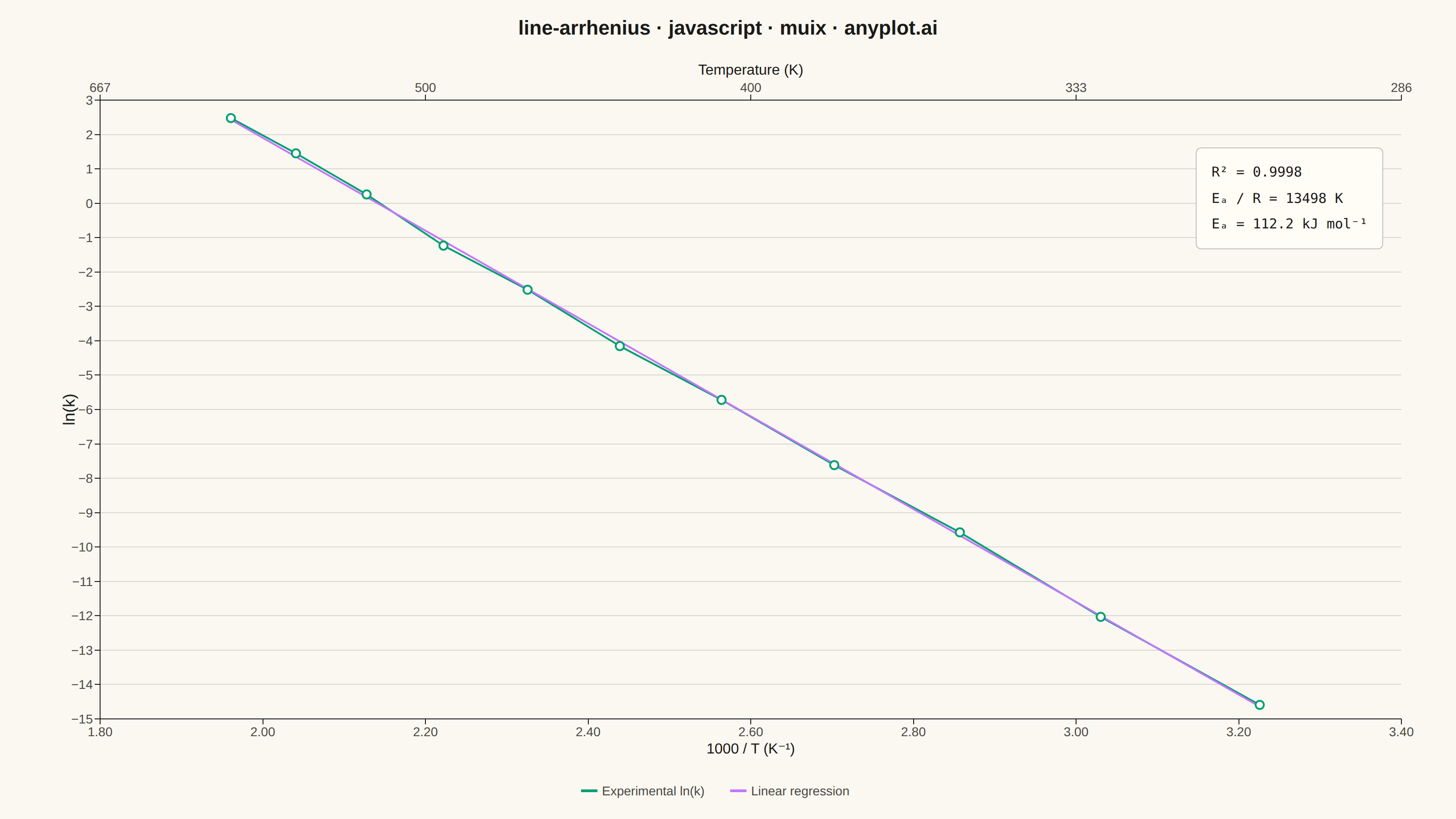
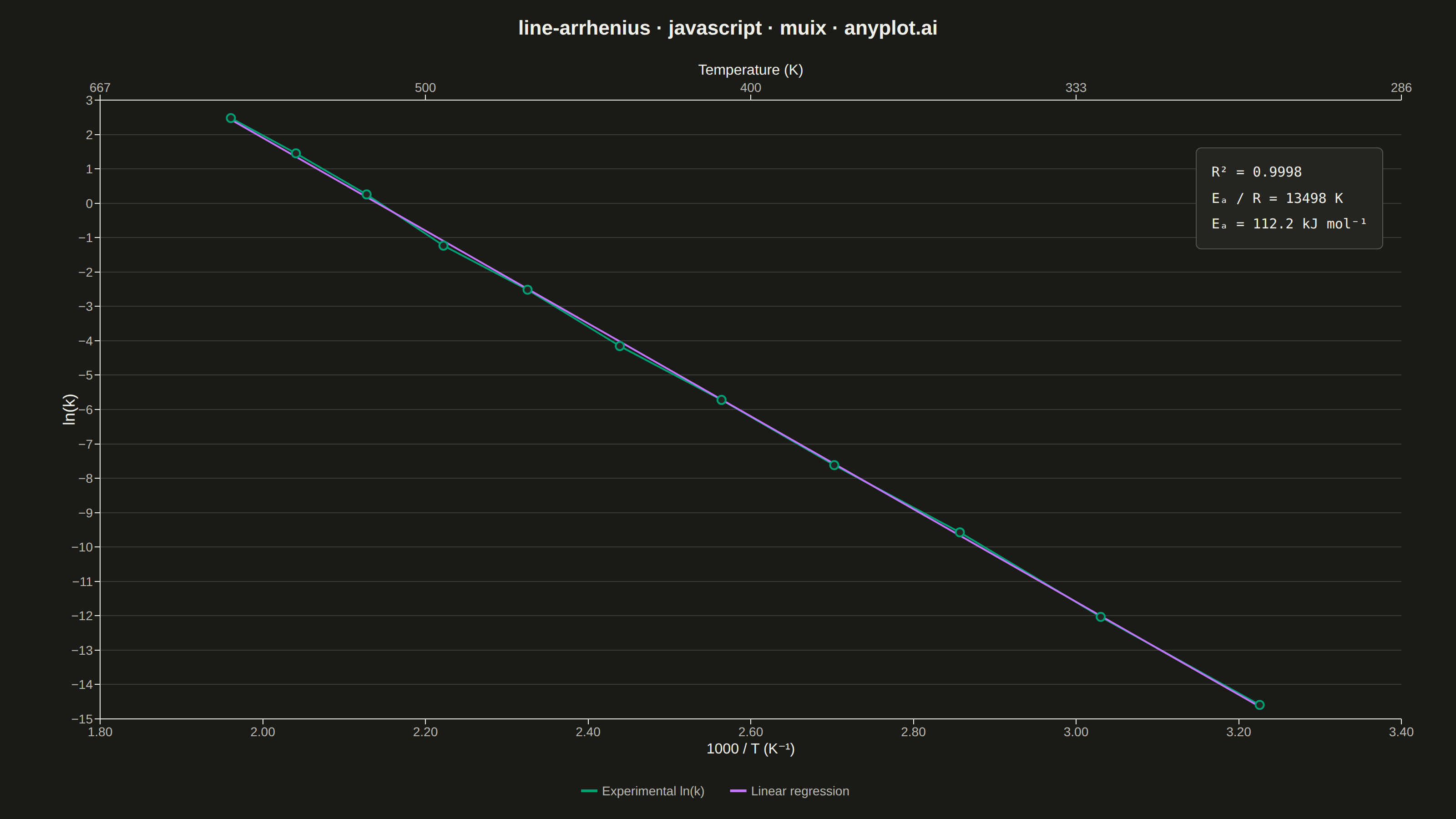
The same plot in 14 other libraries — JavaScript: Chart.js, D3.js, Apache ECharts, Highcharts; Python: Altair, Bokeh, lets-plot, Matplotlib, Plotly, plotnine, Pygal, Seaborn; R: ggplot2; Julia: Makie.jl. Compare all 15 side by side: Arrhenius Plot for Reaction Kinetics in Python, R, Julia and JavaScript.
An Arrhenius plot displays ln(k) versus 1/T to determine the activation energy of a chemical reaction from experimental rate constant data. The Arrhenius equation predicts a linear relationship on this transformed scale, where the slope equals -Ea/R (activation energy divided by the gas constant). This visualization is fundamental in physical chemistry and chemical engineering for characterizing reaction kinetics and comparing catalytic performance.
// anyplot.ai
// line-arrhenius: Arrhenius Plot for Reaction Kinetics
// Library: muix 7.29.1 | JavaScript 22.22.3
// Quality: 88/100 | Created: 2026-06-24
//# anyplot-orientation: landscape
// anyplot.ai
// line-arrhenius: Arrhenius Plot for Reaction Kinetics
// Library: MUI X Charts | React | Node 22
// License: @mui/x-charts — MIT (community). Pro/Premium are out of scope.
// Quality: pending | Created: 2026-06-24

import { LineChart } from "@mui/x-charts/LineChart";
import Box from "@mui/material/Box";
import Typography from "@mui/material/Typography";

const t = window.ANYPLOT_TOKENS;
const sz = window.ANYPLOT_SIZE;

// LCG for deterministic noise (no Math.random — banned in workflow)
let lcgSeed = 42;
function nextLcg() {
  lcgSeed = (Math.imul(lcgSeed, 1664525) + 1013904223) >>> 0;
  return lcgSeed / 4294967296;
}

// Synthetic Arrhenius data — NO₂ thermal decomposition (2NO₂ → 2NO + O₂)
const R_GAS = 8.314;    // J/(mol·K)
const Ea_true = 111000; // J/mol (~111 kJ/mol — literature value)
const lnA = 28.55;      // ln(2.5 × 10¹² s⁻¹) pre-exponential factor

const temps_K = [310, 330, 350, 370, 390, 410, 430, 450, 470, 490, 510];
const xData = temps_K.map((T) => parseFloat((1000 / T).toFixed(4)));
const yData = temps_K.map((T) => {
  const lnK_true = lnA - Ea_true / (R_GAS * T);
  return parseFloat((lnK_true + (nextLcg() - 0.5) * 0.3).toFixed(4));
});

// Linear regression: ln(k) = intercept + slope × (1000/T)
const n = xData.length;
const sumX = xData.reduce((a, b) => a + b, 0);
const sumY = yData.reduce((a, b) => a + b, 0);
const sumXY = xData.reduce((s, x, i) => s + x * yData[i], 0);
const sumX2 = xData.reduce((s, x) => s + x * x, 0);
const slope = (n * sumXY - sumX * sumY) / (n * sumX2 - sumX * sumX);
const intercept = (sumY - slope * sumX) / n;

const yMean = sumY / n;
const ssRes = yData.reduce(
  (s, y, i) => s + (y - (slope * xData[i] + intercept)) ** 2,
  0
);
const ssTot = yData.reduce((s, y) => s + (y - yMean) ** 2, 0);
const r2 = 1 - ssRes / ssTot;

// slope = -Ea / (R × 1000)  →  Ea = -slope × R × 1000
const Ea_kJ = (-slope * R_GAS).toFixed(1);   // kJ/mol
const EaR_K = (-slope * 1000).toFixed(0);     // Ea/R in K

const regData = xData.map((x) =>
  parseFloat((slope * x + intercept).toFixed(4))
);

export default function Chart() {
  return (
    <Box sx={{ position: "relative", width: sz.width, height: sz.height }}>
      {/* Chart title */}
      <Typography
        sx={{
          position: "absolute",
          top: 14,
          left: 0,
          right: 0,
          textAlign: "center",
          color: t.ink,
          fontSize: 22,
          fontWeight: 600,
          zIndex: 1,
          pointerEvents: "none",
        }}
      >
        line-arrhenius · javascript · muix · anyplot.ai
      </Typography>

      <LineChart
        width={sz.width}
        height={sz.height}
        skipAnimation
        margin={{ top: 110, bottom: 110, left: 110, right: 60 }}
        colors={[t.palette[0], t.palette[1]]}
        grid={{ horizontal: true }}
        xAxis={[
          {
            id: "invT",
            data: xData,
            label: "1000 / T  (K⁻¹)",
            valueFormatter: (v) => v.toFixed(2),
            scaleType: "linear",
            position: "bottom",
            tickNumber: 7,
            tickLabelStyle: { fontSize: 14, fill: t.inkSoft },
            labelStyle: { fontSize: 16, fill: t.ink },
          },
          {
            id: "tempK",
            data: xData,
            label: "Temperature (K)",
            valueFormatter: (v) => `${Math.round(1000 / v)}`,
            scaleType: "linear",
            position: "top",
            tickNumber: 5,
            tickLabelStyle: { fontSize: 14, fill: t.inkSoft },
            labelStyle: { fontSize: 16, fill: t.ink },
          },
        ]}
        yAxis={[
          {
            id: "lnk",
            label: "ln(k)",
            labelStyle: { fontSize: 18, fill: t.ink },
            tickLabelStyle: { fontSize: 14, fill: t.inkSoft },
          },
        ]}
        series={[
          {
            id: "experimental",
            data: yData,
            label: "Experimental ln(k)",
            showMark: true,
            curve: "linear",
            xAxisKey: "invT",
          },
          {
            id: "regression",
            data: regData,
            label: "Linear regression",
            showMark: false,
            curve: "linear",
            xAxisKey: "invT",
          },
        ]}
        topAxis="tempK"
        bottomAxis="invT"
        leftAxis="lnk"
        rightAxis={null}
        slotProps={{
          legend: {
            position: { vertical: "bottom", horizontal: "middle" },
            direction: "row",
            itemMarkWidth: 18,
            itemMarkHeight: 3,
            itemGap: 28,
            labelStyle: { fontSize: 14, fill: t.inkSoft },
          },
        }}
      />

      {/* Regression statistics annotation */}
      <Box
        sx={{
          position: "absolute",
          top: "18%",
          right: "5%",
          bgcolor: t.elevatedBg,
          px: 2,
          py: 1.5,
          borderRadius: 1.5,
          border: `1px solid ${t.inkSoft}55`,
          zIndex: 2,
        }}
      >
        <Typography
          sx={{ color: t.ink, fontSize: 15, fontFamily: "monospace", lineHeight: 1.9 }}
        >
          R² = {r2.toFixed(4)}
        </Typography>
        <Typography
          sx={{ color: t.ink, fontSize: 15, fontFamily: "monospace", lineHeight: 1.9 }}
        >
          Eₐ / R = {EaR_K} K
        </Typography>
        <Typography
          sx={{ color: t.ink, fontSize: 15, fontFamily: "monospace", lineHeight: 1.9 }}
        >
          Eₐ = {Ea_kJ} kJ mol⁻¹
        </Typography>
      </Box>
    </Box>
  );
}
Runnable source as JSON, for any HTTP client: https://api.anyplot.ai/specs/line-arrhenius/muix/code. Any spec id and library id listed in llms-full.txt fit the same URL shape; every URL below is complete and callable.
{
  "spec_id": "line-arrhenius",
  "language": "javascript",
  "library": "muix",
  "page": "https://anyplot.ai/line-arrhenius/javascript/muix",
  "hub": "https://anyplot.ai/line-arrhenius",
  "code_json": "https://api.anyplot.ai/specs/line-arrhenius/muix/code",
  "spec_json": "https://api.anyplot.ai/specs/line-arrhenius",
  "render_light_png": "https://storage.googleapis.com/anyplot-images/plots/line-arrhenius/javascript/muix/plot-light.png",
  "render_dark_png": "https://storage.googleapis.com/anyplot-images/plots/line-arrhenius/javascript/muix/plot-dark.png",
  "interactive_light_html": "https://storage.googleapis.com/anyplot-images/plots/line-arrhenius/javascript/muix/plot-light.html",
  "interactive_dark_html": "https://storage.googleapis.com/anyplot-images/plots/line-arrhenius/javascript/muix/plot-dark.html",
  "quality_score": 88.0,
  "license": "MIT",
  "guide": "https://anyplot.ai/llms.txt"
}
Part of Arrhenius Plot for Reaction Kinetics on anyplot.ai.