The same plot in 14 other libraries — JavaScript: Chart.js, Apache ECharts, Highcharts, MUI X Charts; Python: Altair, Bokeh, lets-plot, Matplotlib, Plotly, plotnine, Pygal, Seaborn; R: ggplot2; Julia: Makie.jl. Compare all 15 side by side: Arrhenius Plot for Reaction Kinetics in Python, R, Julia and JavaScript.
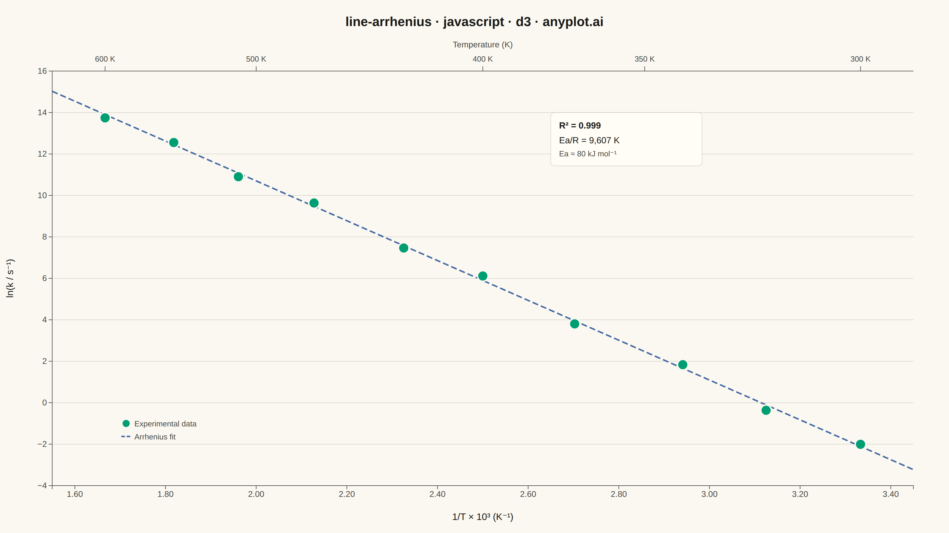
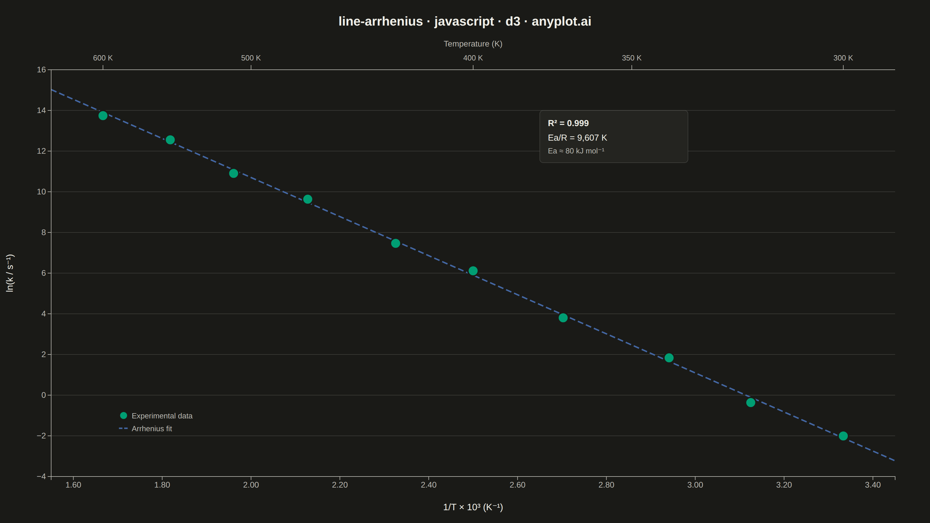
An Arrhenius plot displays ln(k) versus 1/T to determine the activation energy of a chemical reaction from experimental rate constant data. The Arrhenius equation predicts a linear relationship on this transformed scale, where the slope equals -Ea/R (activation energy divided by the gas constant). This visualization is fundamental in physical chemistry and chemical engineering for characterizing reaction kinetics and comparing catalytic performance.
// anyplot.ai
// line-arrhenius: Arrhenius Plot for Reaction Kinetics
// Library: d3 7.9.0 | JavaScript 22.22.3
// Quality: 90/100 | Created: 2026-06-24

const t = window.ANYPLOT_TOKENS;
const { width, height } = window.ANYPLOT_SIZE;

const margin = { top: 120, right: 60, bottom: 80, left: 88 };
const iw = width - margin.left - margin.right;
const ih = height - margin.top - margin.bottom;

// N2O decomposition kinetics — 10 experimental measurements (Ea ≈ 80 kJ/mol, A ≈ 1×10¹³ s⁻¹)
// x = 1000/T (10⁻³ K⁻¹), y = ln(k / s⁻¹); noise added to simulate real experiments
const data = [
  { temp: 300, x: 1000 / 300, y: -2.006 },
  { temp: 320, x: 1000 / 320, y: -0.366 },
  { temp: 340, x: 1000 / 340, y:  1.834 },
  { temp: 370, x: 1000 / 370, y:  3.804 },
  { temp: 400, x: 1000 / 400, y:  6.114 },
  { temp: 430, x: 1000 / 430, y:  7.464 },
  { temp: 470, x: 1000 / 470, y:  9.634 },
  { temp: 510, x: 1000 / 510, y: 10.904 },
  { temp: 550, x: 1000 / 550, y: 12.554 },
  { temp: 600, x: 1000 / 600, y: 13.744 },
];

// Pre-computed Arrhenius linear regression: ln(k) = slope·(1000/T) + intercept
const regSlope     = -9.607;   // units: (10⁻³ K⁻¹)⁻¹
const regIntercept = 29.915;   // ln(A)
const r2           = 0.999;
const eaOverR      = 9607;     // K  (= −slope × 1000)
const ea_kJmol     = 80;       // kJ mol⁻¹

const xDomain = [1.55, 3.45];
const yDomain = [-4, 16];

// SVG
const svg = d3.select("#container")
  .append("svg")
  .attr("width", width)
  .attr("height", height);

const g = svg.append("g")
  .attr("transform", `translate(${margin.left},${margin.top})`);

// Scales
const xScale = d3.scaleLinear().domain(xDomain).range([0, iw]);
const yScale = d3.scaleLinear().domain(yDomain).range([ih, 0]);

// Y-axis grid lines (horizontal, subtle)
yScale.ticks(10).forEach(tick => {
  g.append("line")
    .attr("x1", 0).attr("x2", iw)
    .attr("y1", yScale(tick)).attr("y2", yScale(tick))
    .attr("stroke", t.grid)
    .attr("stroke-width", 1);
});

// Regression line — Imprint blue (palette[2]), dashed
g.append("path")
  .datum([
    [xDomain[0], regSlope * xDomain[0] + regIntercept],
    [xDomain[1], regSlope * xDomain[1] + regIntercept],
  ])
  .attr("d", d3.line().x(d => xScale(d[0])).y(d => yScale(d[1])))
  .attr("fill", "none")
  .attr("stroke", t.palette[2])
  .attr("stroke-width", 2.5)
  .attr("stroke-dasharray", "10,5");

// Data points — Imprint brand green (palette[0]), drawn on top of regression line
g.selectAll(".dot")
  .data(data)
  .join("circle")
  .attr("cx", d => xScale(d.x))
  .attr("cy", d => yScale(d.y))
  .attr("r", 9)
  .attr("fill", t.palette[0])
  .attr("stroke", t.pageBg)
  .attr("stroke-width", 2.5);

// Primary X axis (bottom)
const xAxisEl = g.append("g")
  .attr("transform", `translate(0,${ih})`)
  .call(d3.axisBottom(xScale).ticks(8).tickFormat(d3.format(".2f")));
xAxisEl.selectAll("text").attr("fill", t.inkSoft).style("font-size", "14px");
xAxisEl.selectAll("line").attr("stroke", t.inkSoft);
xAxisEl.select(".domain").attr("stroke", t.inkSoft);

// Y axis (left)
const yAxisEl = g.append("g")
  .call(d3.axisLeft(yScale).ticks(10));
yAxisEl.selectAll("text").attr("fill", t.inkSoft).style("font-size", "14px");
yAxisEl.selectAll("line").attr("stroke", t.inkSoft);
yAxisEl.select(".domain").attr("stroke", t.inkSoft);

// Secondary x-axis at top of plot area — Temperature (K) reference ticks
const tempTicks = [300, 350, 400, 500, 600];
const secG = g.append("g");

secG.append("line")
  .attr("x1", 0).attr("x2", iw)
  .attr("y1", 0).attr("y2", 0)
  .attr("stroke", t.inkSoft)
  .attr("stroke-width", 1);

tempTicks.forEach(temp => {
  const xp = xScale(1000 / temp);
  secG.append("line")
    .attr("x1", xp).attr("x2", xp)
    .attr("y1", 0).attr("y2", -8)
    .attr("stroke", t.inkSoft)
    .attr("stroke-width", 1);
  secG.append("text")
    .attr("x", xp).attr("y", -16)
    .attr("text-anchor", "middle")
    .attr("fill", t.inkSoft)
    .style("font-size", "13px")
    .text(`${temp} K`);
});

// Secondary axis header label
svg.append("text")
  .attr("x", margin.left + iw / 2)
  .attr("y", margin.top - 40)
  .attr("text-anchor", "middle")
  .attr("fill", t.inkSoft)
  .style("font-size", "14px")
  .text("Temperature (K)");

// X axis label
svg.append("text")
  .attr("x", margin.left + iw / 2)
  .attr("y", height - 22)
  .attr("text-anchor", "middle")
  .attr("fill", t.ink)
  .style("font-size", "16px")
  .text("1/T × 10³  (K⁻¹)");

// Y axis label (rotated)
svg.append("text")
  .attr("transform", "rotate(-90)")
  .attr("x", -(margin.top + ih / 2))
  .attr("y", 22)
  .attr("text-anchor", "middle")
  .attr("fill", t.ink)
  .style("font-size", "16px")
  .text("ln(k / s⁻¹)");

// Annotation box — upper-right area of plot (empty: high 1/T region, high y is unoccupied)
const boxX = xScale(2.65);
const boxY = yScale(14.0);
const boxW = 255;
const boxH = 90;

g.append("rect")
  .attr("x", boxX).attr("y", boxY)
  .attr("width", boxW).attr("height", boxH)
  .attr("fill", t.elevatedBg)
  .attr("stroke", t.grid)
  .attr("stroke-width", 1)
  .attr("rx", 6);

g.append("text")
  .attr("x", boxX + 14).attr("y", boxY + 27)
  .attr("fill", t.ink)
  .style("font-size", "15px")
  .style("font-weight", "600")
  .text(`R² = ${r2.toFixed(3)}`);

g.append("text")
  .attr("x", boxX + 14).attr("y", boxY + 52)
  .attr("fill", t.ink)
  .style("font-size", "15px")
  .text(`Ea/R = ${eaOverR.toLocaleString()} K`);

g.append("text")
  .attr("x", boxX + 14).attr("y", boxY + 74)
  .attr("fill", t.inkSoft)
  .style("font-size", "13px")
  .text(`Ea ≈ ${ea_kJmol} kJ mol⁻¹`);

// Small legend in bottom-left (T≈590K region, ln(k)≈−1 — no data or line here)
const legX = xScale(1.7);
const legY = yScale(-1.0);

g.append("circle")
  .attr("cx", legX + 10).attr("cy", legY)
  .attr("r", 7)
  .attr("fill", t.palette[0])
  .attr("stroke", t.pageBg)
  .attr("stroke-width", 2);
g.append("text")
  .attr("x", legX + 24).attr("y", legY + 5)
  .attr("fill", t.inkSoft)
  .style("font-size", "13px")
  .text("Experimental data");

g.append("line")
  .attr("x1", legX + 2).attr("x2", legX + 18)
  .attr("y1", legY + 22).attr("y2", legY + 22)
  .attr("stroke", t.palette[2])
  .attr("stroke-width", 2.5)
  .attr("stroke-dasharray", "6,3");
g.append("text")
  .attr("x", legX + 24).attr("y", legY + 27)
  .attr("fill", t.inkSoft)
  .style("font-size", "13px")
  .text("Arrhenius fit");

// Title
svg.append("text")
  .attr("x", width / 2)
  .attr("y", 44)
  .attr("text-anchor", "middle")
  .attr("fill", t.ink)
  .style("font-size", "22px")
  .style("font-weight", "600")
  .text("line-arrhenius · javascript · d3 · anyplot.ai");
Runnable source as JSON, for any HTTP client: https://api.anyplot.ai/specs/line-arrhenius/d3/code. Any spec id and library id listed in llms-full.txt fit the same URL shape; every URL below is complete and callable.
{
  "spec_id": "line-arrhenius",
  "language": "javascript",
  "library": "d3",
  "page": "https://anyplot.ai/line-arrhenius/javascript/d3",
  "hub": "https://anyplot.ai/line-arrhenius",
  "code_json": "https://api.anyplot.ai/specs/line-arrhenius/d3/code",
  "spec_json": "https://api.anyplot.ai/specs/line-arrhenius",
  "render_light_png": "https://storage.googleapis.com/anyplot-images/plots/line-arrhenius/javascript/d3/plot-light.png",
  "render_dark_png": "https://storage.googleapis.com/anyplot-images/plots/line-arrhenius/javascript/d3/plot-dark.png",
  "interactive_light_html": "https://storage.googleapis.com/anyplot-images/plots/line-arrhenius/javascript/d3/plot-light.html",
  "interactive_dark_html": "https://storage.googleapis.com/anyplot-images/plots/line-arrhenius/javascript/d3/plot-dark.html",
  "quality_score": 90.0,
  "license": "MIT",
  "guide": "https://anyplot.ai/llms.txt"
}
Part of Arrhenius Plot for Reaction Kinetics on anyplot.ai.