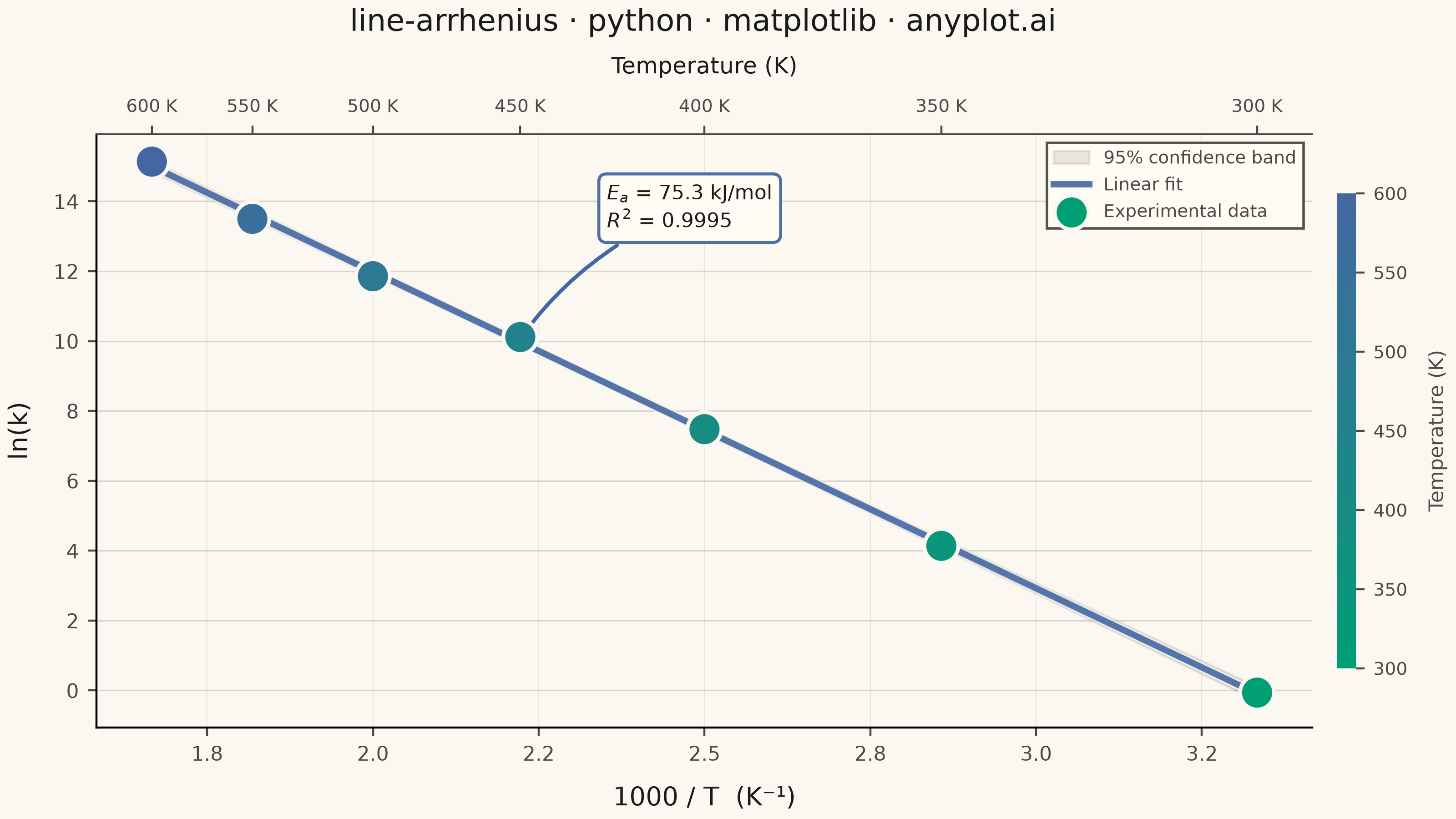
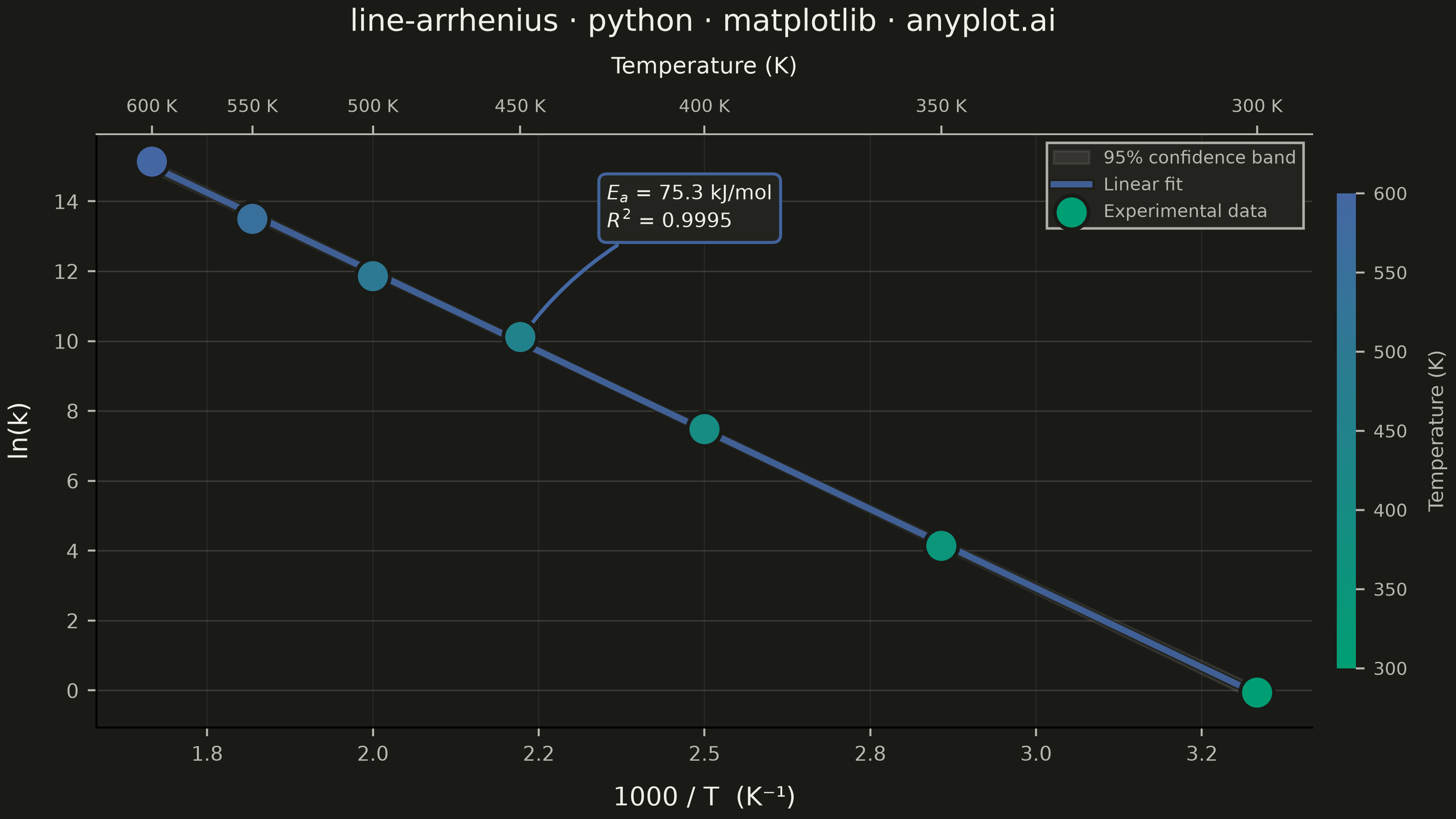
An Arrhenius plot displays ln(k) versus 1/T to determine the activation energy of a chemical reaction from experimental rate constant data. The Arrhenius equation predicts a linear relationship on this transformed scale, where the slope equals -Ea/R (activation energy divided by the gas constant). This visualization is fundamental in physical chemistry and chemical engineering for characterizing reaction kinetics and comparing catalytic performance.
""" anyplot.ai
line-arrhenius: Arrhenius Plot for Reaction Kinetics
Library: matplotlib 3.11.0 | Python 3.13.14
Quality: 90/100 | Updated: 2026-06-24
"""

import os

import matplotlib.patheffects as pe
import matplotlib.pyplot as plt
import matplotlib.ticker as ticker
import numpy as np
from matplotlib.colors import LinearSegmentedColormap


# Theme tokens
THEME = os.getenv("ANYPLOT_THEME", "light")
PAGE_BG = "#FAF8F1" if THEME == "light" else "#1A1A17"
ELEVATED_BG = "#FFFDF6" if THEME == "light" else "#242420"
INK = "#1A1A17" if THEME == "light" else "#F0EFE8"
INK_SOFT = "#4A4A44" if THEME == "light" else "#B8B7B0"
INK_MUTED = "#6B6A63" if THEME == "light" else "#A8A79F"

# Imprint sequential colormap for continuous temperature data (#009E73 → #4467A3)
imprint_seq = LinearSegmentedColormap.from_list("imprint_seq", ["#009E73", "#4467A3"])

# Data — first-order decomposition reaction rate constants at various temperatures
temperature_K = np.array([300, 350, 400, 450, 500, 550, 600])
activation_energy_true = 75000  # J/mol (75 kJ/mol)
R_gas = 8.314  # J/(mol·K)
pre_exponential = 1e13  # s⁻¹

np.random.seed(42)
rate_constant_k = (
    pre_exponential
    * np.exp(-activation_energy_true / (R_gas * temperature_K))
    * np.exp(np.random.normal(0, 0.15, len(temperature_K)))
)

inv_temperature = 1000 / temperature_K  # 1000/T for cleaner x-axis values
ln_k = np.log(rate_constant_k)

# Linear regression
coeffs = np.polyfit(1 / temperature_K, ln_k, 1)
slope, intercept = coeffs
ln_k_predicted = slope * (1 / temperature_K) + intercept
ss_res = np.sum((ln_k - ln_k_predicted) ** 2)
ss_tot = np.sum((ln_k - np.mean(ln_k)) ** 2)
r_squared = 1 - ss_res / ss_tot
activation_energy = -slope * R_gas / 1000  # kJ/mol

inv_temp_fit = np.linspace(1 / temperature_K.max(), 1 / temperature_K.min(), 200)
ln_k_fit = slope * inv_temp_fit + intercept

# Confidence band (±2 SE)
residual_se = np.sqrt(ss_res / (len(temperature_K) - 2))
inv_T_arr = 1 / temperature_K
x_mean = np.mean(inv_T_arr)
s_xx = np.sum((inv_T_arr - x_mean) ** 2)
se_fit = residual_se * np.sqrt(1 / len(inv_T_arr) + (inv_temp_fit - x_mean) ** 2 / s_xx)

# Plot — figsize=(8,4.5) dpi=400 → exactly 3200×1800 px
fig, ax = plt.subplots(figsize=(8, 4.5), dpi=400, facecolor=PAGE_BG, constrained_layout=True)
ax.set_facecolor(PAGE_BG)

# 95% confidence band
ax.fill_between(
    inv_temp_fit * 1000,
    ln_k_fit - 2 * se_fit,
    ln_k_fit + 2 * se_fit,
    color=INK_SOFT,
    alpha=0.12,
    zorder=1,
    label="95% confidence band",
)

# Regression line (Imprint blue #4467A3)
ax.plot(
    inv_temp_fit * 1000,
    ln_k_fit,
    color="#4467A3",
    linewidth=2.5,
    alpha=0.90,
    label="Linear fit",
    zorder=2,
    path_effects=[pe.withStroke(linewidth=4, foreground=PAGE_BG, alpha=0.5)],
)

# Data points — Imprint sequential colormap by temperature
scatter = ax.scatter(
    inv_temperature,
    ln_k,
    s=180,
    c=temperature_K,
    cmap=imprint_seq,
    vmin=temperature_K.min(),
    vmax=temperature_K.max(),
    edgecolors=PAGE_BG,
    linewidth=1.5,
    zorder=4,
    label="Experimental data",
)

# Colorbar — temperature scale
cbar = fig.colorbar(scatter, ax=ax, pad=0.02, aspect=25, shrink=0.80)
cbar.set_label("Temperature (K)", fontsize=8, labelpad=8, color=INK_SOFT)
cbar.ax.tick_params(labelsize=7, colors=INK_SOFT)
cbar.outline.set_visible(False)

# Annotation — Ea and R²
mid_idx = len(inv_temp_fit) // 3
ax.annotate(
    f"$E_a$ = {activation_energy:.1f} kJ/mol\n$R^2$ = {r_squared:.4f}",
    xy=(inv_temp_fit[mid_idx] * 1000, ln_k_fit[mid_idx]),
    xytext=(35, 45),
    textcoords="offset points",
    fontsize=8,
    fontweight="medium",
    color=INK,
    bbox={
        "boxstyle": "round,pad=0.4",
        "facecolor": ELEVATED_BG,
        "edgecolor": "#4467A3",
        "alpha": 0.95,
        "linewidth": 1.2,
    },
    arrowprops={"arrowstyle": "-|>", "color": "#4467A3", "lw": 1.5, "connectionstyle": "arc3,rad=0.15"},
)

# Style
title = "line-arrhenius · python · matplotlib · anyplot.ai"
title_fontsize = max(8, round(12 * 67 / len(title))) if len(title) > 67 else 12

ax.set_xlabel("1000 / T  (K⁻¹)", fontsize=10, labelpad=8, color=INK)
ax.set_ylabel("ln(k)", fontsize=10, labelpad=8, color=INK)
ax.set_title(
    title,
    fontsize=title_fontsize,
    fontweight="medium",
    pad=10,
    color=INK,
    path_effects=[pe.withStroke(linewidth=3, foreground=PAGE_BG, alpha=0.8)],
)
ax.tick_params(axis="both", labelsize=8, colors=INK_SOFT, labelcolor=INK_SOFT)
ax.spines["top"].set_visible(False)
ax.spines["right"].set_visible(False)
ax.spines["left"].set_linewidth(0.7)
ax.spines["left"].set_color(INK_SOFT)
ax.spines["bottom"].set_linewidth(0.7)
ax.spines["bottom"].set_color(INK_SOFT)
ax.yaxis.grid(True, alpha=0.15, linewidth=0.6, color=INK)
ax.xaxis.grid(True, alpha=0.08, linewidth=0.4, color=INK)
ax.xaxis.set_major_formatter(ticker.FormatStrFormatter("%.1f"))

# Legend
leg = ax.legend(fontsize=7, framealpha=0.95, edgecolor=INK_SOFT, loc="upper right", fancybox=False)
if leg:
    leg.get_frame().set_facecolor(ELEVATED_BG)
    plt.setp(leg.get_texts(), color=INK_SOFT)

# Secondary x-axis — temperature in K
ax2 = ax.twiny()
ax2.set_xlim(ax.get_xlim())
temp_ticks = np.array([600, 550, 500, 450, 400, 350, 300])
tick_positions = 1000 / temp_ticks
ax2.set_xticks(tick_positions)
ax2.set_xticklabels([f"{t} K" for t in temp_ticks], fontsize=7)
ax2.set_xlabel("Temperature (K)", fontsize=9, labelpad=10, color=INK)
ax2.spines["right"].set_visible(False)
ax2.spines["top"].set_linewidth(0.7)
ax2.spines["top"].set_color(INK_SOFT)
ax2.tick_params(axis="x", labelsize=7, colors=INK_SOFT, labelcolor=INK_SOFT)

# Save — no bbox_inches so figsize×dpi → exactly 3200×1800
plt.savefig(f"plot-{THEME}.png", dpi=400, facecolor=PAGE_BG)
plt.close()
Runnable source as JSON, for any HTTP client: https://api.anyplot.ai/specs/line-arrhenius/matplotlib/code. Any spec id and library id listed in llms-full.txt fit the same URL shape; every URL below is complete and callable.
{
  "spec_id": "line-arrhenius",
  "language": "python",
  "library": "matplotlib",
  "page": "https://anyplot.ai/line-arrhenius/python/matplotlib",
  "hub": "https://anyplot.ai/line-arrhenius",
  "code_json": "https://api.anyplot.ai/specs/line-arrhenius/matplotlib/code",
  "spec_json": "https://api.anyplot.ai/specs/line-arrhenius",
  "render_light_png": "https://storage.googleapis.com/anyplot-images/plots/line-arrhenius/python/matplotlib/plot-light.png",
  "render_dark_png": "https://storage.googleapis.com/anyplot-images/plots/line-arrhenius/python/matplotlib/plot-dark.png",
  "quality_score": 90.0,
  "license": "MIT",
  "guide": "https://anyplot.ai/llms.txt"
}
Part of Arrhenius Plot for Reaction Kinetics on anyplot.ai.