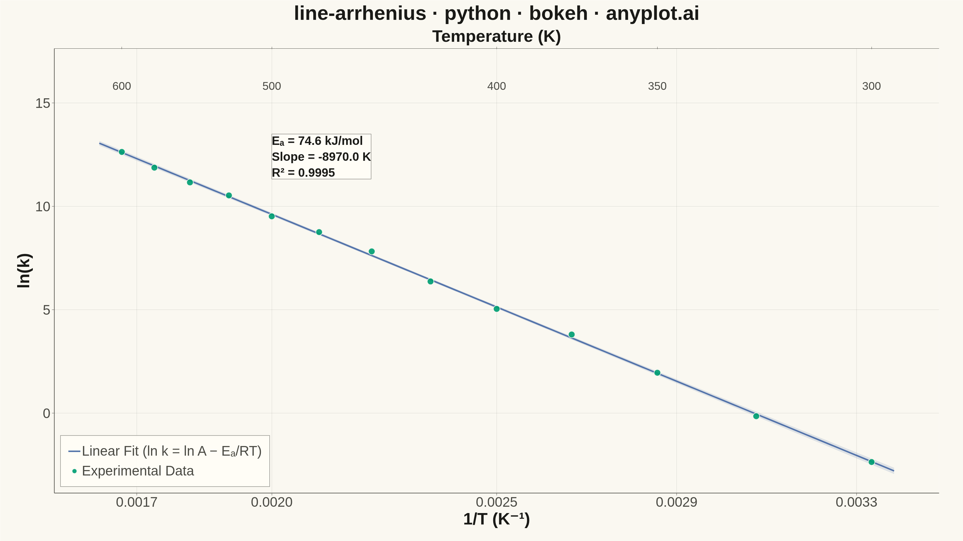
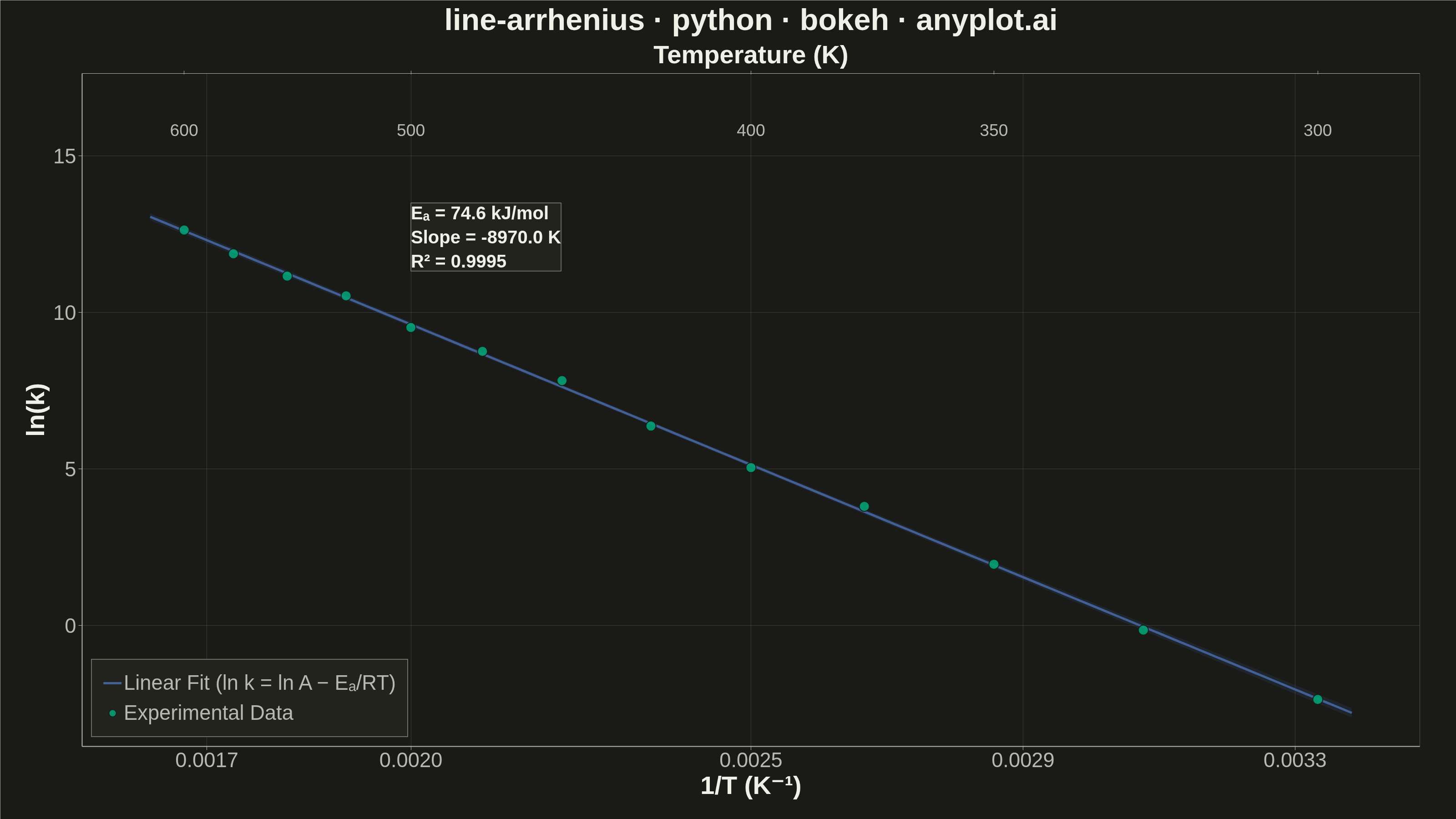
An Arrhenius plot displays ln(k) versus 1/T to determine the activation energy of a chemical reaction from experimental rate constant data. The Arrhenius equation predicts a linear relationship on this transformed scale, where the slope equals -Ea/R (activation energy divided by the gas constant). This visualization is fundamental in physical chemistry and chemical engineering for characterizing reaction kinetics and comparing catalytic performance.
""" anyplot.ai
line-arrhenius: Arrhenius Plot for Reaction Kinetics
Library: bokeh 3.9.1 | Python 3.13.14
Quality: 87/100 | Updated: 2026-06-24
"""

import os
import sys
import time
from pathlib import Path


# Prevent this file (bokeh.py) from shadowing the installed bokeh package when
# Python prepends the script's own directory to sys.path on startup.
_here = os.path.dirname(os.path.abspath(__file__))
sys.path = [p for p in sys.path if os.path.abspath(p or ".") != _here]

import numpy as np
from bokeh.io import output_file, save
from bokeh.models import ColumnDataSource, HoverTool, Label, LinearAxis, NumeralTickFormatter
from bokeh.models.tickers import FixedTicker
from bokeh.plotting import figure
from bokeh.resources import CDN
from scipy import stats
from selenium import webdriver
from selenium.webdriver.chrome.options import Options


# Theme tokens (Imprint palette + theme-adaptive chrome)
THEME = os.getenv("ANYPLOT_THEME", "light")
PAGE_BG = "#FAF8F1" if THEME == "light" else "#1A1A17"
ELEVATED_BG = "#FFFDF6" if THEME == "light" else "#242420"
INK = "#1A1A17" if THEME == "light" else "#F0EFE8"
INK_SOFT = "#4A4A44" if THEME == "light" else "#B8B7B0"
INK_MUTED = "#6B6A63" if THEME == "light" else "#A8A79F"

# Imprint categorical palette — positions used here
BRAND = "#009E73"  # position 1 — data points
LINE_COLOR = "#4467A3"  # position 3 — regression line

# Data — first-order decomposition reaction rate constants at various temperatures
np.random.seed(42)
temperature_K = np.array([300, 325, 350, 375, 400, 425, 450, 475, 500, 525, 550, 575, 600])
activation_energy = 75000  # J/mol (typical organic decomposition)
R_gas = 8.314  # gas constant J/(mol·K)
pre_exponential = 1e12  # s^-1

# Generate rate constants from Arrhenius equation with experimental noise
ln_k_true = np.log(pre_exponential) - activation_energy / (R_gas * temperature_K)
noise = np.random.normal(0, 0.15, len(temperature_K))
ln_k = ln_k_true + noise
inv_T = 1.0 / temperature_K

# Linear regression: ln(k) = ln(A) - Ea/R * (1/T)
slope, intercept, r_value, p_value, std_err = stats.linregress(inv_T, ln_k)
r_squared = r_value**2
Ea_fitted = -slope * R_gas  # activation energy from slope

# Regression line
inv_T_line = np.linspace(inv_T.min() - 0.00005, inv_T.max() + 0.00005, 200)
ln_k_line = slope * inv_T_line + intercept

# 95% confidence interval band around regression
n_pts = len(inv_T)
x_mean = inv_T.mean()
Sxx = np.sum((inv_T - x_mean) ** 2)
s_e = np.sqrt(np.sum((ln_k - (slope * inv_T + intercept)) ** 2) / (n_pts - 2))
t_val = stats.t.ppf(0.975, df=n_pts - 2)
se_band = s_e * np.sqrt(1.0 / n_pts + (inv_T_line - x_mean) ** 2 / Sxx)
ci_upper = ln_k_line + t_val * se_band
ci_lower = ln_k_line - t_val * se_band

# Data sources
scatter_source = ColumnDataSource(
    data={
        "inv_T": inv_T,
        "ln_k": ln_k,
        "T_K": temperature_K,
        "inv_T_fmt": [f"{x:.4f}" for x in inv_T],
        "ln_k_fmt": [f"{y:.2f}" for y in ln_k],
    }
)
line_source = ColumnDataSource(data={"inv_T": inv_T_line, "ln_k": ln_k_line})
ci_source = ColumnDataSource(data={"inv_T": inv_T_line, "ci_upper": ci_upper, "ci_lower": ci_lower})

# Title — canonical format; length=43 chars < 67, use default 50pt
TITLE = "line-arrhenius · python · bokeh · anyplot.ai"

# Figure — canvas exactly 3200×1800 (landscape); toolbar_location=None for correct PNG size
p = figure(
    width=3200,
    height=1800,
    title=TITLE,
    x_axis_label="1/T (K⁻¹)",
    y_axis_label="ln(k)",
    x_range=(inv_T.min() - 0.00015, inv_T.max() + 0.00015),
    y_range=(ln_k.min() - 1.5, ln_k.max() + 5.0),
    toolbar_location=None,
    min_border_bottom=160,
    min_border_left=180,
    min_border_top=110,
    min_border_right=80,
)

# Background
p.background_fill_color = PAGE_BG
p.border_fill_color = PAGE_BG
p.outline_line_alpha = 0  # L-shaped frame: remove box outline, keep axis lines

# 95% confidence band behind regression line
p.varea(x="inv_T", y1="ci_lower", y2="ci_upper", source=ci_source, fill_color=LINE_COLOR, fill_alpha=0.15)

# Regression line (Imprint position 3 — blue)
p.line(
    "inv_T",
    "ln_k",
    source=line_source,
    line_color=LINE_COLOR,
    line_width=5,
    line_alpha=0.9,
    legend_label="Linear Fit (ln k = ln A − Eₐ/RT)",
)

# Data points (Imprint position 1 — brand green)
scatter_renderer = p.scatter(
    "inv_T",
    "ln_k",
    source=scatter_source,
    size=22,
    color=BRAND,
    alpha=0.92,
    line_color=PAGE_BG,
    line_width=2,
    legend_label="Experimental Data",
)

# HoverTool
hover = HoverTool(
    renderers=[scatter_renderer],
    tooltips=[("Temperature", "@T_K K"), ("1/T", "@inv_T_fmt K⁻¹"), ("ln(k)", "@ln_k_fmt")],
    mode="mouse",
)
p.add_tools(hover)

# Annotation: slope, activation energy, R²
eq_text = f"Eₐ = {Ea_fitted / 1000:.1f} kJ/mol\nSlope = {slope:.1f} K\nR² = {r_squared:.4f}"
eq_label = Label(
    x=inv_T[8],
    y=ln_k[6] + 3.5,
    text=eq_text,
    text_font_size="30pt",
    text_color=INK,
    text_font_style="bold",
    background_fill_color=ELEVATED_BG,
    background_fill_alpha=0.92,
    border_line_color=INK_SOFT,
    border_line_alpha=0.5,
    border_line_width=2,
)
p.add_layout(eq_label)

# Secondary x-axis for temperature (above)
temp_label_values = [300, 350, 400, 500, 600]
temp_tick_positions = [1.0 / t for t in temp_label_values]
temp_axis = LinearAxis(
    axis_label="Temperature (K)",
    axis_label_text_font_size="42pt",
    axis_label_text_color=INK,
    axis_label_text_font_style="bold",
    major_label_text_font_size="34pt",
    major_label_text_color=INK_SOFT,
    ticker=FixedTicker(ticks=temp_tick_positions),
    major_tick_line_color=INK_SOFT,
    minor_tick_line_color=None,
    axis_line_color=INK_SOFT,
)
p.add_layout(temp_axis, "above")

# Temperature tick labels via Label annotations (inside plot area, near top)
for t_val in temp_label_values:
    inv_t_val = 1.0 / t_val
    temp_label = Label(
        x=inv_t_val,
        y=ln_k.max() + 3.0,
        text=str(t_val),
        text_font_size="28pt",
        text_color=INK_SOFT,
        text_align="center",
        text_baseline="bottom",
    )
    p.add_layout(temp_label)

# Axis references — after add_layout(above): xaxis[0]=top, xaxis[1]=bottom
bottom_ax = p.xaxis[1]
top_ax = p.xaxis[0]

# Bottom x-axis: fixed ticks with formatting
bottom_ticks = [round(1.0 / t, 4) for t in [600, 500, 400, 350, 300]]
bottom_ax.ticker = FixedTicker(ticks=bottom_ticks)
bottom_ax.formatter = NumeralTickFormatter(format="0.0000")

# Hide top axis tick labels (Label annotations used instead)
top_ax.major_label_text_font_size = "0pt"

# Title styling
p.title.text_font_size = "50pt"
p.title.text_color = INK
p.title.align = "center"
p.title.text_font_style = "bold"

# Bottom x-axis styling
bottom_ax.axis_label_text_font_size = "42pt"
bottom_ax.axis_label_text_color = INK
bottom_ax.axis_label_text_font_style = "bold"
bottom_ax.major_label_text_font_size = "34pt"
bottom_ax.major_label_text_color = INK_SOFT

# Y-axis styling
p.yaxis.axis_label_text_font_size = "42pt"
p.yaxis.axis_label_text_color = INK
p.yaxis.axis_label_text_font_style = "bold"
p.yaxis.major_label_text_font_size = "34pt"
p.yaxis.major_label_text_color = INK_SOFT

# Legend styling
p.legend.label_text_font_size = "34pt"
p.legend.label_text_color = INK_SOFT
p.legend.location = "bottom_left"
p.legend.background_fill_color = ELEVATED_BG
p.legend.background_fill_alpha = 0.92
p.legend.border_line_color = INK_SOFT
p.legend.border_line_alpha = 0.5
p.legend.border_line_width = 2
p.legend.glyph_height = 40
p.legend.glyph_width = 40
p.legend.padding = 25
p.legend.spacing = 14
p.legend.margin = 20

# Grid — subtle, 15% opacity
p.xgrid.grid_line_color = INK
p.ygrid.grid_line_color = INK
p.xgrid.grid_line_alpha = 0.15
p.ygrid.grid_line_alpha = 0.15

# Axis lines and ticks
for ax in [bottom_ax, p.yaxis[0]]:
    ax.axis_line_color = INK_SOFT
    ax.axis_line_width = 2
    ax.minor_tick_line_color = None
    ax.major_tick_line_color = INK_SOFT
    ax.major_tick_out = 8
    ax.major_tick_in = 0

# Save interactive HTML artifact
output_file(f"plot-{THEME}.html")
save(p, resources=CDN, title="Arrhenius Plot for Reaction Kinetics")

# Screenshot with headless Chrome (Selenium 4).
# Use CDP Emulation.setDeviceMetricsOverride so the viewport is exactly W×H
# regardless of any browser-chrome offset that would otherwise clip the canvas.
W, H = 3200, 1800
opts = Options()
for arg in (
    "--headless=new",
    "--no-sandbox",
    "--disable-dev-shm-usage",
    "--disable-gpu",
    f"--window-size={W},{H}",
    "--hide-scrollbars",
):
    opts.add_argument(arg)
driver = webdriver.Chrome(options=opts)
driver.execute_cdp_cmd(
    "Emulation.setDeviceMetricsOverride", {"width": W, "height": H, "deviceScaleFactor": 1, "mobile": False}
)
driver.get(f"file://{Path(f'plot-{THEME}.html').resolve()}")
time.sleep(3)
driver.save_screenshot(f"plot-{THEME}.png")
driver.quit()
Runnable source as JSON, for any HTTP client: https://api.anyplot.ai/specs/line-arrhenius/bokeh/code. Any spec id and library id listed in llms-full.txt fit the same URL shape; every URL below is complete and callable.
{
  "spec_id": "line-arrhenius",
  "language": "python",
  "library": "bokeh",
  "page": "https://anyplot.ai/line-arrhenius/python/bokeh",
  "hub": "https://anyplot.ai/line-arrhenius",
  "code_json": "https://api.anyplot.ai/specs/line-arrhenius/bokeh/code",
  "spec_json": "https://api.anyplot.ai/specs/line-arrhenius",
  "render_light_png": "https://storage.googleapis.com/anyplot-images/plots/line-arrhenius/python/bokeh/plot-light.png",
  "render_dark_png": "https://storage.googleapis.com/anyplot-images/plots/line-arrhenius/python/bokeh/plot-dark.png",
  "interactive_light_html": "https://storage.googleapis.com/anyplot-images/plots/line-arrhenius/python/bokeh/plot-light.html",
  "interactive_dark_html": "https://storage.googleapis.com/anyplot-images/plots/line-arrhenius/python/bokeh/plot-dark.html",
  "quality_score": 87.0,
  "license": "MIT",
  "guide": "https://anyplot.ai/llms.txt"
}
Part of Arrhenius Plot for Reaction Kinetics on anyplot.ai.