The same plot in 14 other libraries — Python: Altair, Bokeh, lets-plot, Matplotlib, Plotly, plotnine, Pygal, Seaborn; R: ggplot2; JavaScript: Chart.js, D3.js, Apache ECharts, Highcharts, MUI X Charts. Compare all 15 side by side: Arrhenius Plot for Reaction Kinetics in Python, R, Julia and JavaScript.
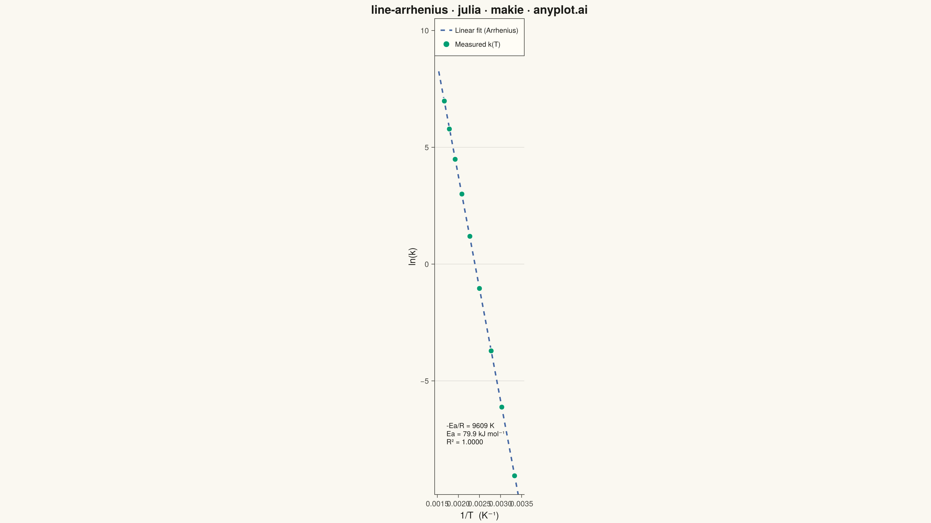
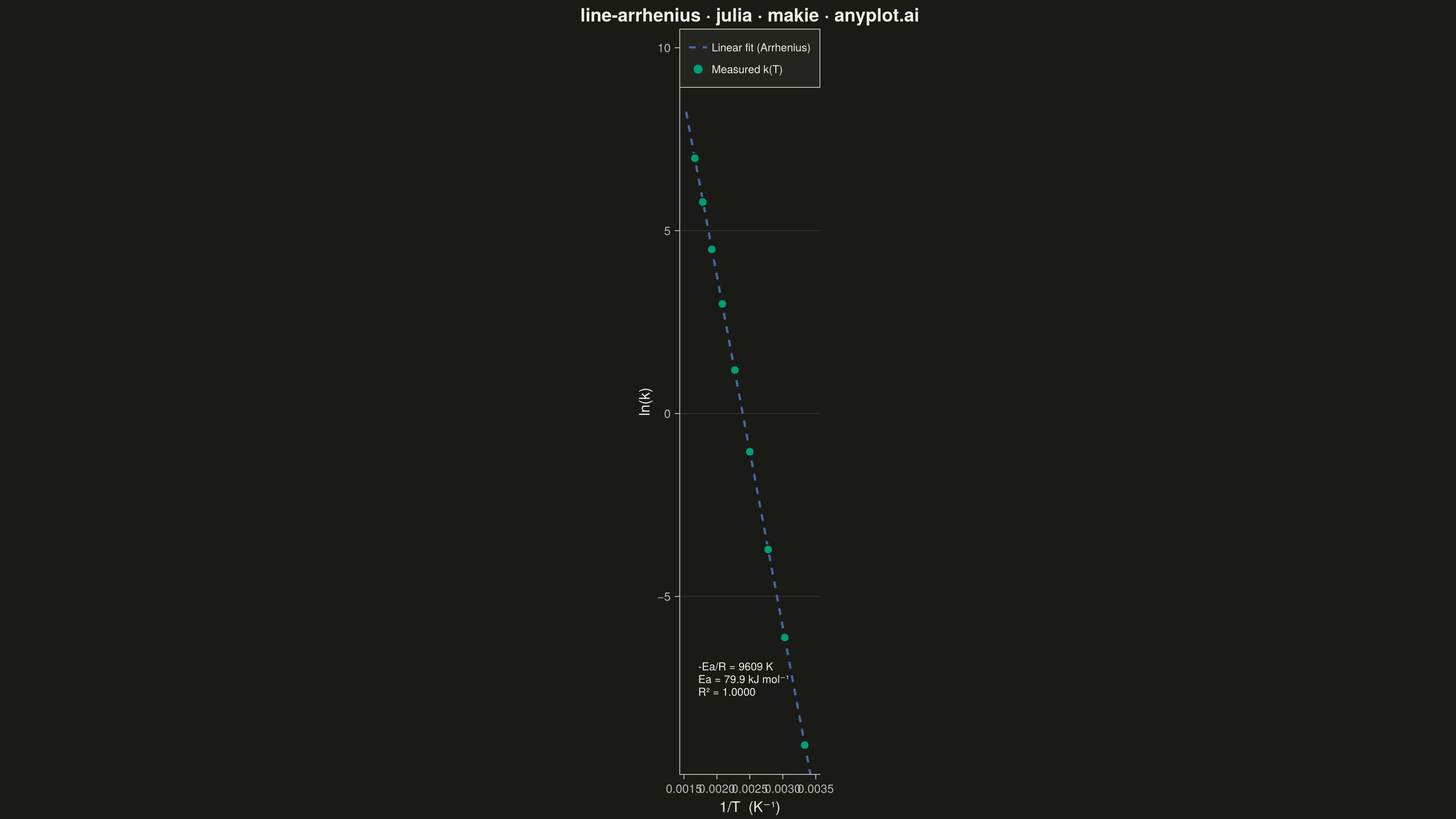
An Arrhenius plot displays ln(k) versus 1/T to determine the activation energy of a chemical reaction from experimental rate constant data. The Arrhenius equation predicts a linear relationship on this transformed scale, where the slope equals -Ea/R (activation energy divided by the gas constant). This visualization is fundamental in physical chemistry and chemical engineering for characterizing reaction kinetics and comparing catalytic performance.
# anyplot.ai
# line-arrhenius: Arrhenius Plot for Reaction Kinetics
# Library: makie 0.22.10 | Julia 1.11.9
# Quality: 84/100 | Created: 2026-06-24

using CairoMakie
using Colors
using Random
using Statistics
using Printf

Random.seed!(42)

# Theme tokens
const THEME       = get(ENV, "ANYPLOT_THEME", "light")
const PAGE_BG     = THEME == "light" ? colorant"#FAF8F1" : colorant"#1A1A17"
const ELEVATED_BG = THEME == "light" ? colorant"#FFFDF6" : colorant"#242420"
const INK         = THEME == "light" ? colorant"#1A1A17" : colorant"#F0EFE8"
const INK_SOFT    = THEME == "light" ? colorant"#4A4A44" : colorant"#B8B7B0"

const IMPRINT_PALETTE = [
    colorant"#009E73", colorant"#C475FD", colorant"#4467A3", colorant"#BD8233",
    colorant"#AE3030", colorant"#2ABCCD", colorant"#954477", colorant"#99B314",
]

# Arrhenius data: first-order thermal decomposition
# k = A * exp(-Ea / R / T),  Ea = 80 kJ/mol,  A = 1e10 s⁻¹
const R_GAS = 8.314     # J mol⁻¹ K⁻¹
const EA    = 80_000.0  # J mol⁻¹
const A_PRE = 1.0e10    # s⁻¹

temperatures_K = [300.0, 330.0, 360.0, 400.0, 440.0, 480.0, 520.0, 560.0, 600.0]
k_ideal        = A_PRE .* exp.(-EA ./ (R_GAS .* temperatures_K))
rate_constants = k_ideal .* (1.0 .+ 0.04 .* randn(length(temperatures_K)))

# Arrhenius linearisation using 1000/T on x-axis (conventional; avoids tiny tick numbers)
inv_T_scaled = 1000.0 ./ temperatures_K  # values ≈ 1.67 – 3.33
ln_k         = log.(rate_constants)

# Linear regression: ln(k) = slope * (1000/T) + intercept
x_bar = mean(inv_T_scaled)
y_bar = mean(ln_k)
slope     = sum((inv_T_scaled .- x_bar) .* (ln_k .- y_bar)) /
            sum((inv_T_scaled .- x_bar).^2)
intercept = y_bar - slope * x_bar

ln_k_fit = slope .* inv_T_scaled .+ intercept
r_sq     = 1.0 - sum((ln_k .- ln_k_fit).^2) / sum((ln_k .- y_bar).^2)

# Ea from slope: since x = 1000/T, slope × 1000 = -Ea/R
ea_kJmol = -slope * R_GAS  # ≈ 79.9 kJ/mol

# Extended regression line
margin = 0.08 * (maximum(inv_T_scaled) - minimum(inv_T_scaled))
x_fit  = collect(range(minimum(inv_T_scaled) - margin,
                       maximum(inv_T_scaled) + margin; length = 200))
y_fit  = slope .* x_fit .+ intercept

# 95% confidence band (t_{0.025, df=7} = 2.365)
n_pts   = length(inv_T_scaled)
sse     = sum((ln_k .- ln_k_fit).^2)
s2      = sse / (n_pts - 2)
Sxx     = sum((inv_T_scaled .- x_bar).^2)
t_crit  = 2.365
se_band = sqrt.(s2 .* (1.0 / n_pts .+ (x_fit .- x_bar).^2 ./ Sxx))
y_upper = y_fit .+ t_crit .* se_band
y_lower = y_fit .- t_crit .* se_band

title_str  = "line-arrhenius · julia · makie · anyplot.ai"
title_size = length(title_str) > 67 ? max(14, round(Int, 20 * 67 / length(title_str))) : 20

fig = Figure(
    size            = (1600, 900),
    fontsize        = 14,
    backgroundcolor = PAGE_BG,
)

ax = Axis(
    fig[1, 1];
    title              = title_str,
    titlesize          = title_size,
    titlecolor         = INK,
    xlabel             = "10³/T  (K⁻¹)",
    ylabel             = "ln(k)",
    xlabelsize         = 16,
    ylabelsize         = 16,
    xticklabelsize     = 13,
    yticklabelsize     = 13,
    xlabelcolor        = INK,
    ylabelcolor        = INK,
    xticklabelcolor    = INK_SOFT,
    yticklabelcolor    = INK_SOFT,
    xtickcolor         = INK_SOFT,
    ytickcolor         = INK_SOFT,
    backgroundcolor    = PAGE_BG,
    topspinevisible    = false,
    rightspinevisible  = false,
    leftspinecolor     = INK_SOFT,
    bottomspinecolor   = INK_SOFT,
    xgridvisible       = false,
    ygridvisible       = true,
    xminorgridvisible  = false,
    yminorgridvisible  = false,
    ygridcolor         = RGBAf(INK.r, INK.g, INK.b, 0.12),
    xticks             = LinearTicks(4),
)

# True secondary x-axis: temperature reference in K (overlapping Axis at top)
ax_top = Axis(
    fig[1, 1];
    xaxisposition      = :top,
    yaxisposition      = :right,
    backgroundcolor    = :transparent,
    topspinevisible    = true,
    topspinecolor      = INK_SOFT,
    bottomspinevisible = false,
    leftspinevisible   = false,
    rightspinevisible  = false,
    xgridvisible       = false,
    ygridvisible       = false,
    yticksvisible      = false,
    yticklabelsvisible = false,
    xlabel             = "Temperature (K)",
    xlabelsize         = 13,
    xlabelcolor        = INK_SOFT,
    xticklabelsize     = 11,
    xticklabelcolor    = INK_SOFT,
    xtickcolor         = INK_SOFT,
    xticks             = (
        1000.0 ./ [300.0, 350.0, 400.0, 500.0, 600.0],
        ["300", "350", "400", "500", "600"],
    ),
)
linkxaxes!(ax, ax_top)
linkyaxes!(ax, ax_top)

# Confidence band (Makie band! — highlights fit quality)
band!(ax, x_fit, y_lower, y_upper;
    color = (IMPRINT_PALETTE[3], 0.15),
)

# Regression line (drawn before markers so they render on top)
lines!(ax, x_fit, y_fit;
    color     = IMPRINT_PALETTE[3],
    linewidth = 2.5,
    linestyle = :dash,
    label     = "Linear fit (Arrhenius)",
)

# Experimental data points
scatter!(ax, inv_T_scaled, ln_k;
    color       = IMPRINT_PALETTE[1],
    markersize  = 14,
    strokewidth = 1.5,
    strokecolor = PAGE_BG,
    label       = "Measured k(T)",
)

# Annotation: kinetic parameters — lower-left corner
x_range = maximum(inv_T_scaled) - minimum(inv_T_scaled)
y_range = maximum(ln_k) - minimum(ln_k)
x_ann   = minimum(inv_T_scaled) + 0.03 * x_range
y_ann   = minimum(ln_k) + 0.08 * y_range

text!(ax, x_ann, y_ann;
    text     = @sprintf("-Ea/R = %d K\nEa = %.1f kJ mol⁻¹\nR² = %.4f",
                   round(Int, -slope * 1000.0), ea_kJmol, r_sq),
    color    = INK,
    fontsize = 12,
    align    = (:left, :bottom),
)

axislegend(ax;
    position        = :rt,
    labelsize       = 12,
    framevisible    = true,
    framecolor      = INK_SOFT,
    backgroundcolor = ELEVATED_BG,
    labelcolor      = INK,
)

resize_to_layout!(fig)
save("plot-$(THEME).png", fig; px_per_unit = 2)
Runnable source as JSON, for any HTTP client: https://api.anyplot.ai/specs/line-arrhenius/makie/code. Any spec id and library id listed in llms-full.txt fit the same URL shape; every URL below is complete and callable.
{
  "spec_id": "line-arrhenius",
  "language": "julia",
  "library": "makie",
  "page": "https://anyplot.ai/line-arrhenius/julia/makie",
  "hub": "https://anyplot.ai/line-arrhenius",
  "code_json": "https://api.anyplot.ai/specs/line-arrhenius/makie/code",
  "spec_json": "https://api.anyplot.ai/specs/line-arrhenius",
  "render_light_png": "https://storage.googleapis.com/anyplot-images/plots/line-arrhenius/julia/makie/plot-light.png",
  "render_dark_png": "https://storage.googleapis.com/anyplot-images/plots/line-arrhenius/julia/makie/plot-dark.png",
  "quality_score": 84.0,
  "license": "MIT",
  "guide": "https://anyplot.ai/llms.txt"
}
Part of Arrhenius Plot for Reaction Kinetics on anyplot.ai.