The same plot in 14 other libraries — Python: Altair, Bokeh, lets-plot, Matplotlib, Plotly, plotnine, Pygal, Seaborn; Julia: Makie.jl; JavaScript: Chart.js, D3.js, Apache ECharts, Highcharts, MUI X Charts. Compare all 15 side by side: Arrhenius Plot for Reaction Kinetics in Python, R, Julia and JavaScript.
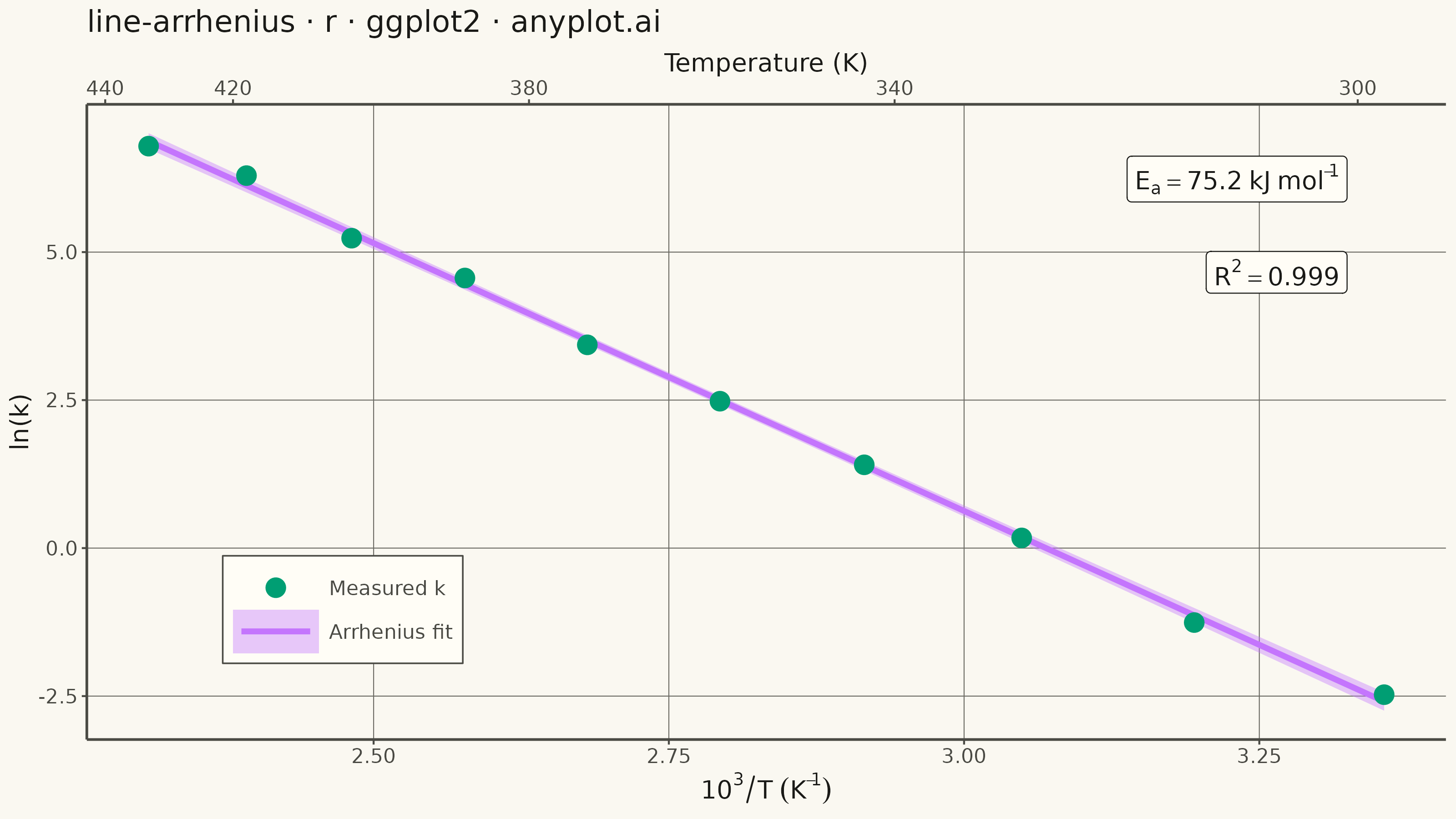
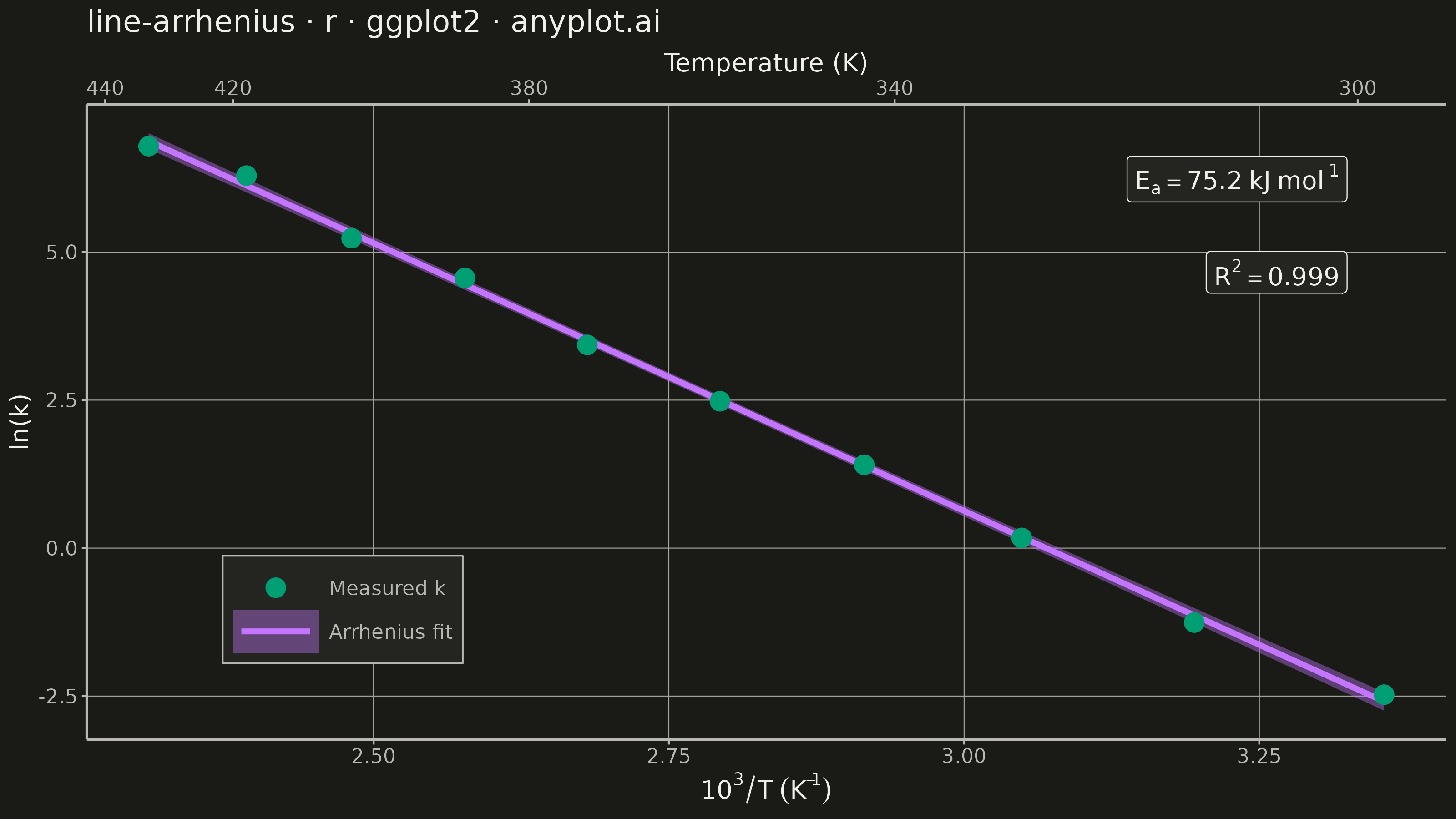
An Arrhenius plot displays ln(k) versus 1/T to determine the activation energy of a chemical reaction from experimental rate constant data. The Arrhenius equation predicts a linear relationship on this transformed scale, where the slope equals -Ea/R (activation energy divided by the gas constant). This visualization is fundamental in physical chemistry and chemical engineering for characterizing reaction kinetics and comparing catalytic performance.
#' anyplot.ai
#' line-arrhenius: Arrhenius Plot for Reaction Kinetics
#' Library: ggplot2 3.5.1 | R 4.4.1
#' Quality: 91/100 | Created: 2026-06-24

library(ggplot2)
library(scales)
library(ragg)

set.seed(42)

# --- Theme tokens -----------------------------------------------------------
THEME       <- Sys.getenv("ANYPLOT_THEME", "light")
PAGE_BG     <- if (THEME == "light") "#FAF8F1" else "#1A1A17"
ELEVATED_BG <- if (THEME == "light") "#FFFDF6" else "#242420"
INK         <- if (THEME == "light") "#1A1A17" else "#F0EFE8"
INK_SOFT    <- if (THEME == "light") "#4A4A44" else "#B8B7B0"
INK_MUTED   <- if (THEME == "light") "#6B6A63" else "#A8A79F"

# Imprint palette (canonical order, theme-independent)
IMPRINT_PALETTE <- c(
    "#009E73", "#C475FD", "#4467A3", "#BD8233",
    "#AE3030", "#2ABCCD", "#954477", "#99B314"
)

# --- Data -------------------------------------------------------------------
# H2O2 catalytic decomposition, Ea ~ 75 kJ/mol
R_gas   <- 8.314   # J/(mol·K)
Ea_true <- 75000   # J/mol
A_pre   <- 1e12    # pre-exponential factor (s⁻¹)

temps_K   <- c(298, 313, 328, 343, 358, 373, 388, 403, 418, 433)
ln_k_true <- log(A_pre) - Ea_true / (R_gas * temps_K)
ln_k      <- ln_k_true + rnorm(length(temps_K), 0, 0.12)
x_1k      <- 1000 / temps_K   # 10³/T  (K⁻¹)

df <- data.frame(x_1k = x_1k, ln_k = ln_k)

# --- Arrhenius fit ----------------------------------------------------------
fit  <- lm(ln_k ~ x_1k, data = df)
b0   <- coef(fit)[["(Intercept)"]]
b1   <- coef(fit)[["x_1k"]]
r_sq <- summary(fit)$r.squared
# slope = -Ea / (R × 1000)  →  Ea [kJ/mol] = -slope × R_gas
Ea_kJ <- -b1 * R_gas

# --- Annotation text (R plotmath) ------------------------------------------
# Annotations in upper-right (above the descending regression line)
x_rng  <- range(x_1k)
y_rng  <- range(df$ln_k)
ann_x  <- x_rng[2] - 0.03 * diff(x_rng)
ann_y1 <- y_rng[2] - 0.06 * diff(y_rng)
ann_y2 <- y_rng[2] - 0.23 * diff(y_rng)

label_ea <- sprintf("E[a] == %.1f~kJ~mol^{-1}", Ea_kJ)
label_r2 <- sprintf("R^2 == %.4f", r_sq)

# Secondary x-axis: temperature in K (440 K covers the full data range up to 433 K)
sec_breaks <- c(300, 340, 380, 420, 440)

# --- Plot -------------------------------------------------------------------
p <- ggplot() +
    geom_smooth(
        data      = df,
        aes(x = x_1k, y = ln_k, color = "Arrhenius fit"),
        method    = "lm",
        formula   = y ~ x,
        se        = TRUE,
        fill      = alpha(IMPRINT_PALETTE[2], 0.15),
        linewidth = 1.1
    ) +
    geom_point(
        data  = df,
        aes(x = x_1k, y = ln_k, color = "Measured k"),
        size  = 3.5,
        shape = 16
    ) +
    annotate(
        "label",
        x = ann_x, y = ann_y1,
        label = label_ea, parse = TRUE,
        hjust = 1, size = 3.5,
        color = INK, fill = ELEVATED_BG, label.size = 0.2
    ) +
    annotate(
        "label",
        x = ann_x, y = ann_y2,
        label = label_r2, parse = TRUE,
        hjust = 1, size = 3.5,
        color = INK, fill = ELEVATED_BG, label.size = 0.2
    ) +
    scale_color_manual(
        name   = NULL,
        values = c(
            "Measured k"    = IMPRINT_PALETTE[1],   # brand green — first series
            "Arrhenius fit" = IMPRINT_PALETTE[2]    # lavender — second series
        ),
        breaks = c("Measured k", "Arrhenius fit")
    ) +
    scale_x_continuous(
        name     = expression(10^3 / T ~ (K^{-1})),
        sec.axis = sec_axis(
            transform = ~ 1000 / .,
            name      = "Temperature (K)",
            breaks    = sec_breaks,
            labels    = as.character(sec_breaks)
        )
    ) +
    labs(
        y     = "ln(k)",
        title = "line-arrhenius · r · ggplot2 · anyplot.ai"
    ) +
    theme_minimal(base_size = 8) +
    theme(
        plot.background      = element_rect(fill = PAGE_BG,    color = PAGE_BG),
        panel.background     = element_rect(fill = PAGE_BG,    color = NA),
        panel.grid.major     = element_line(color = INK_MUTED, linewidth = 0.18),
        panel.grid.minor     = element_blank(),
        panel.border         = element_blank(),
        axis.line.x.bottom   = element_line(color = INK_SOFT,  linewidth = 0.5),
        axis.line.x.top      = element_line(color = INK_SOFT,  linewidth = 0.5),
        axis.line.y.left     = element_line(color = INK_SOFT,  linewidth = 0.5),
        axis.ticks           = element_line(color = INK_SOFT),
        axis.title           = element_text(color = INK,       size = 10),
        axis.text            = element_text(color = INK_SOFT,  size = 8),
        plot.title           = element_text(color = INK,       size = 12, hjust = 0),
        legend.position        = "inside",
        legend.position.inside = c(0.10, 0.12),
        legend.justification   = c(0, 0),
        legend.background    = element_rect(fill = ELEVATED_BG, color = INK_SOFT, linewidth = 0.3),
        legend.text          = element_text(color = INK_SOFT,  size = 8),
        legend.title         = element_blank(),
        legend.key           = element_blank(),
        legend.key.width     = unit(1.2, "cm")
    )

# --- Save -------------------------------------------------------------------
ggsave(
    filename = sprintf("plot-%s.png", THEME),
    plot     = p,
    device   = ragg::agg_png,
    width    = 8,
    height   = 4.5,
    units    = "in",
    dpi      = 400
)
Runnable source as JSON, for any HTTP client: https://api.anyplot.ai/specs/line-arrhenius/ggplot2/code. Any spec id and library id listed in llms-full.txt fit the same URL shape; every URL below is complete and callable.
{
  "spec_id": "line-arrhenius",
  "language": "r",
  "library": "ggplot2",
  "page": "https://anyplot.ai/line-arrhenius/r/ggplot2",
  "hub": "https://anyplot.ai/line-arrhenius",
  "code_json": "https://api.anyplot.ai/specs/line-arrhenius/ggplot2/code",
  "spec_json": "https://api.anyplot.ai/specs/line-arrhenius",
  "render_light_png": "https://storage.googleapis.com/anyplot-images/plots/line-arrhenius/r/ggplot2/plot-light.png",
  "render_dark_png": "https://storage.googleapis.com/anyplot-images/plots/line-arrhenius/r/ggplot2/plot-dark.png",
  "quality_score": 91.0,
  "license": "MIT",
  "guide": "https://anyplot.ai/llms.txt"
}
Part of Arrhenius Plot for Reaction Kinetics on anyplot.ai.