The same plot in 14 other libraries — JavaScript: Chart.js, D3.js, Highcharts, MUI X Charts; Python: Altair, Bokeh, lets-plot, Matplotlib, Plotly, plotnine, Pygal, Seaborn; R: ggplot2; Julia: Makie.jl. Compare all 15 side by side: Arrhenius Plot for Reaction Kinetics in Python, R, Julia and JavaScript.
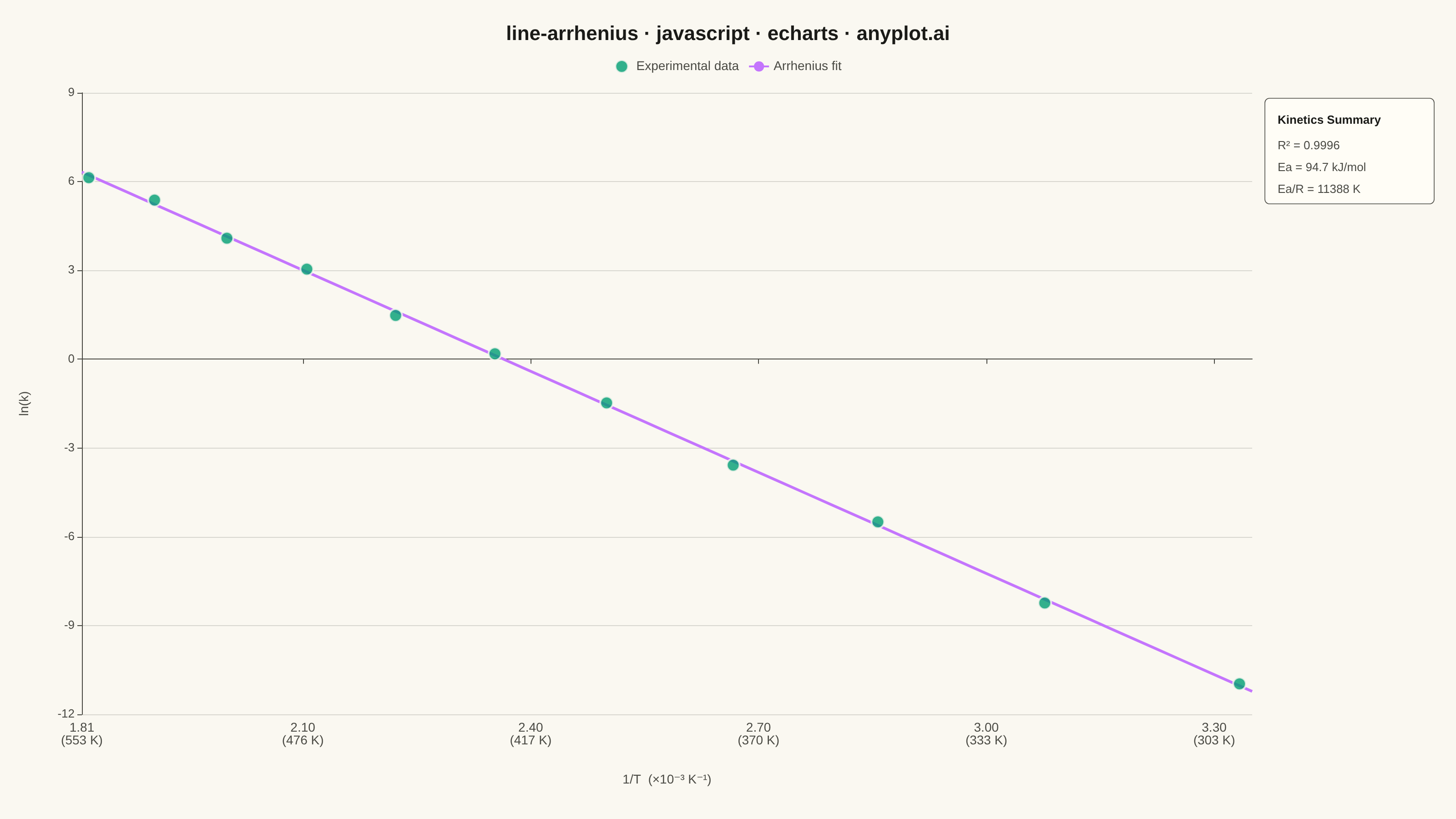
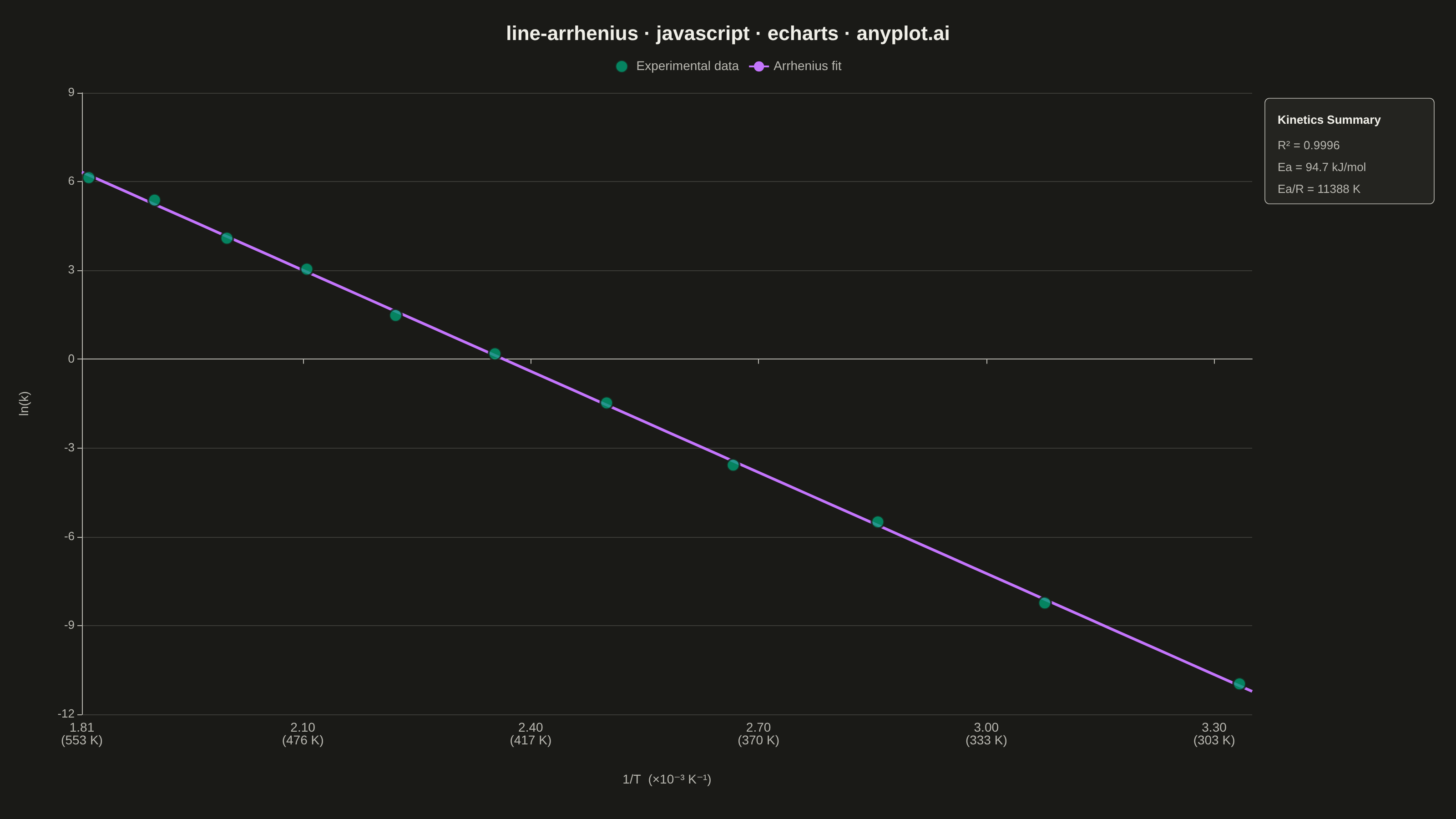
An Arrhenius plot displays ln(k) versus 1/T to determine the activation energy of a chemical reaction from experimental rate constant data. The Arrhenius equation predicts a linear relationship on this transformed scale, where the slope equals -Ea/R (activation energy divided by the gas constant). This visualization is fundamental in physical chemistry and chemical engineering for characterizing reaction kinetics and comparing catalytic performance.
// anyplot.ai
// line-arrhenius: Arrhenius Plot for Reaction Kinetics
// Library: echarts 5.5.1 | JavaScript 22.22.3
// Quality: 90/100 | Created: 2026-06-24
//# anyplot-orientation: landscape

const t = window.ANYPLOT_TOKENS;

// --- Data (deterministic, in-memory) ----------------------------------------
// First-order thermal decomposition of hydrogen peroxide (H₂O₂ → H₂O + ½O₂)
const temps_K = [300, 325, 350, 375, 400, 425, 450, 475, 500, 525, 550];
const R_GAS = 8.314;    // J/(mol·K)
const EA_TRUE = 95000;  // J/mol — activation energy
const LN_A = 27.0;      // ln(A) where A is the pre-exponential factor in s⁻¹

// Deterministic perturbations to simulate experimental measurement scatter
const noise = [0.12, -0.08, 0.15, -0.11, 0.09, 0.07, -0.13, 0.10, -0.06, 0.14, -0.09];
const inv_T = temps_K.map(T => 1 / T);
const ln_k = temps_K.map((T, i) => LN_A - EA_TRUE / (R_GAS * T) + noise[i]);

// Linear regression: ln(k) = slope * (1/T) + intercept  (slope = -Ea/R)
const n = inv_T.length;
const sx = inv_T.reduce((a, b) => a + b, 0);
const sy = ln_k.reduce((a, b) => a + b, 0);
const sxy = inv_T.reduce((a, xi, i) => a + xi * ln_k[i], 0);
const sx2 = inv_T.reduce((a, xi) => a + xi * xi, 0);
const slope = (n * sxy - sx * sy) / (n * sx2 - sx * sx);
const intercept = (sy - slope * sx) / n;

// R² coefficient of determination
const y_mean = sy / n;
const ss_res = ln_k.reduce((a, yi, i) => a + (yi - (slope * inv_T[i] + intercept)) ** 2, 0);
const ss_tot = ln_k.reduce((a, yi) => a + (yi - y_mean) ** 2, 0);
const r_sq = (1 - ss_res / ss_tot).toFixed(4);

// Extracted activation energy from Arrhenius slope: slope = -Ea/R
const Ea_kJ = (-slope * R_GAS / 1000).toFixed(1);
const Ea_over_R = (-slope).toFixed(0);

// Regression line (51 points for smooth rendering, extended beyond data range)
const x_lo = Math.min(...inv_T) * 0.995;
const x_hi = Math.max(...inv_T) * 1.005;
const line_data = Array.from({ length: 51 }, (_, i) => {
  const x = x_lo + (x_hi - x_lo) * i / 50;
  return [x, slope * x + intercept];
});

// --- Init -------------------------------------------------------------------
const chart = echarts.init(document.getElementById("container"));

// --- Option -----------------------------------------------------------------
chart.setOption({
  animation: false,
  color: t.palette,
  backgroundColor: "transparent",
  title: {
    text: "line-arrhenius · javascript · echarts · anyplot.ai",
    left: "center",
    top: 22,
    textStyle: { color: t.ink, fontSize: 22, fontWeight: "bold" }
  },
  legend: {
    data: ["Experimental data", "Arrhenius fit"],
    top: 60,
    textStyle: { color: t.inkSoft, fontSize: 14 },
    itemWidth: 22,
    itemHeight: 14
  },
  tooltip: {
    trigger: "item",
    backgroundColor: t.elevatedBg,
    borderColor: t.inkSoft,
    textStyle: { color: t.ink, fontSize: 13 },
    formatter: function(params) {
      if (params.seriesType === "scatter") {
        const T = Math.round(1 / params.data[0]);
        return (
          "T = " + T + " K<br>" +
          "1/T = " + (params.data[0] * 1000).toFixed(3) + " ×10⁻³ K⁻¹<br>" +
          "ln(k) = " + params.data[1].toFixed(3)
        );
      }
      return "";
    }
  },
  grid: { left: 90, right: 224, top: 102, bottom: 115 },
  xAxis: {
    type: "value",
    name: "1/T  (×10⁻³ K⁻¹)",
    nameLocation: "middle",
    nameGap: 65,
    nameTextStyle: { color: t.inkSoft, fontSize: 14 },
    min: x_lo,
    max: x_hi,
    axisLabel: {
      color: t.inkSoft,
      fontSize: 14,
      formatter: function(val) {
        return (val * 1000).toFixed(2) + "\n(" + Math.round(1 / val) + " K)";
      }
    },
    axisLine: { lineStyle: { color: t.inkSoft } },
    splitLine: { show: false },
    axisTick: { lineStyle: { color: t.inkSoft } }
  },
  yAxis: {
    type: "value",
    name: "ln(k)",
    nameLocation: "middle",
    nameGap: 56,
    nameTextStyle: { color: t.inkSoft, fontSize: 14 },
    axisLabel: { color: t.inkSoft, fontSize: 13 },
    axisLine: { lineStyle: { color: t.inkSoft } },
    splitLine: { lineStyle: { color: t.grid } },
    axisTick: { lineStyle: { color: t.inkSoft } }
  },
  series: [
    {
      name: "Experimental data",
      type: "scatter",
      symbolSize: 14,
      data: inv_T.map((x, i) => [x, ln_k[i]]),
      itemStyle: {
        color: t.palette[0],
        borderColor: t.pageBg,
        borderWidth: 2
      },
      z: 10
    },
    {
      name: "Arrhenius fit",
      type: "line",
      data: line_data,
      lineStyle: { color: t.palette[1], width: 3 },
      itemStyle: { color: t.palette[1] },
      symbol: "none",
      smooth: false,
      z: 5
    }
  ],
  graphic: [
    {
      type: "group",
      x: 1390,
      y: 108,
      children: [
        {
          type: "rect",
          shape: { x: 0, y: 0, width: 186, height: 116, r: 5 },
          style: {
            fill: t.elevatedBg,
            stroke: t.inkSoft,
            lineWidth: 0.8
          }
        },
        {
          type: "text",
          x: 14,
          y: 18,
          style: {
            text: "Kinetics Summary",
            fill: t.ink,
            fontSize: 13,
            fontWeight: "bold"
          }
        },
        {
          type: "text",
          x: 14,
          y: 46,
          style: {
            text: "R² = " + r_sq,
            fill: t.inkSoft,
            fontSize: 13
          }
        },
        {
          type: "text",
          x: 14,
          y: 70,
          style: {
            text: "Ea = " + Ea_kJ + " kJ/mol",
            fill: t.inkSoft,
            fontSize: 13
          }
        },
        {
          type: "text",
          x: 14,
          y: 94,
          style: {
            text: "Ea/R = " + Ea_over_R + " K",
            fill: t.inkSoft,
            fontSize: 13
          }
        }
      ]
    }
  ]
});
Runnable source as JSON, for any HTTP client: https://api.anyplot.ai/specs/line-arrhenius/echarts/code. Any spec id and library id listed in llms-full.txt fit the same URL shape; every URL below is complete and callable.
{
  "spec_id": "line-arrhenius",
  "language": "javascript",
  "library": "echarts",
  "page": "https://anyplot.ai/line-arrhenius/javascript/echarts",
  "hub": "https://anyplot.ai/line-arrhenius",
  "code_json": "https://api.anyplot.ai/specs/line-arrhenius/echarts/code",
  "spec_json": "https://api.anyplot.ai/specs/line-arrhenius",
  "render_light_png": "https://storage.googleapis.com/anyplot-images/plots/line-arrhenius/javascript/echarts/plot-light.png",
  "render_dark_png": "https://storage.googleapis.com/anyplot-images/plots/line-arrhenius/javascript/echarts/plot-dark.png",
  "interactive_light_html": "https://storage.googleapis.com/anyplot-images/plots/line-arrhenius/javascript/echarts/plot-light.html",
  "interactive_dark_html": "https://storage.googleapis.com/anyplot-images/plots/line-arrhenius/javascript/echarts/plot-dark.html",
  "quality_score": 90.0,
  "license": "MIT",
  "guide": "https://anyplot.ai/llms.txt"
}
Part of Arrhenius Plot for Reaction Kinetics on anyplot.ai.