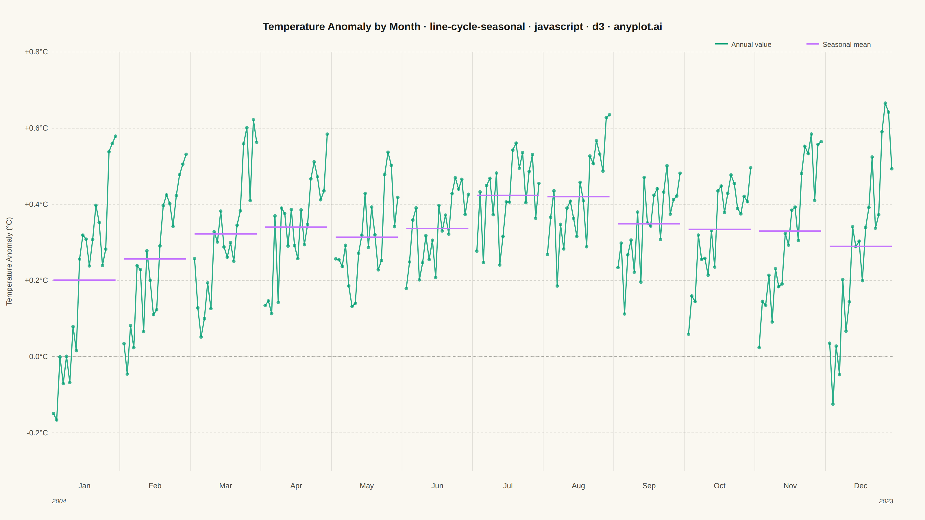
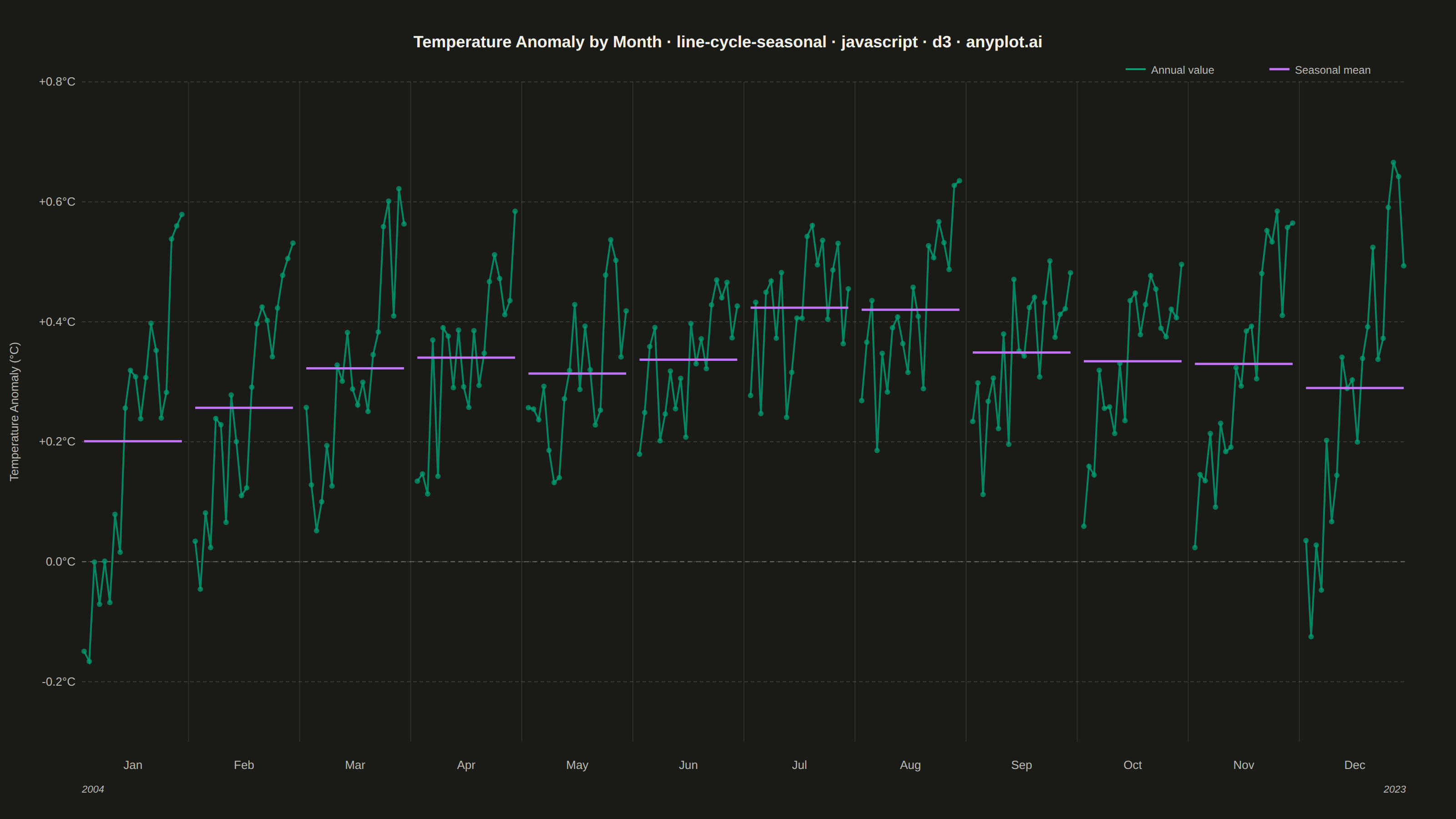
A cycle plot, also known as a seasonal subseries plot (introduced by William Cleveland), separates the seasonal pattern of a time series from the trend within each season. The series is split by seasonal period (e.g. one group per month or weekday); within each group the values are drawn in chronological order as a small line, and a horizontal reference line marks that group's mean. Comparing the mean lines across groups reveals the seasonal effect, while the slope of each subseries reveals the trend within that season — two patterns that are entangled in a standard time series plot.
// anyplot.ai
// line-cycle-seasonal: Cycle Plot (Seasonal Subseries)
// Library: d3 7.9.0 | JavaScript 22.22.3
// Quality: 89/100 | Created: 2026-06-15
//# anyplot-orientation: landscape
// anyplot.ai
// line-cycle-seasonal: Cycle Plot (Seasonal Subseries)
// Library: d3 7.9.0 | JavaScript 22
// Quality: pending | Created: 2026-06-15

const t = window.ANYPLOT_TOKENS;
const { width, height } = window.ANYPLOT_SIZE;

const margin = { top: 90, right: 55, bottom: 85, left: 90 };
const iw = width - margin.left - margin.right;
const ih = height - margin.top - margin.bottom;

// --- Data: monthly temperature anomaly (°C), 2004–2023 ----------------------
const MONTHS = ["Jan","Feb","Mar","Apr","May","Jun","Jul","Aug","Sep","Oct","Nov","Dec"];
const N_YEARS = 20;
const START_YEAR = 2004;

let _seed = 42;
const rng = () => { _seed = (_seed * 1664525 + 1013904223) & 0xffffffff; return (_seed >>> 0) / 0xffffffff; };

// Seasonal baseline anomaly (°C) and total warming over the 20-year window per month
const BASE = [-0.08, 0.02, 0.12, 0.18, 0.15, 0.24, 0.30, 0.28, 0.20, 0.12, 0.04, -0.02];
const WARM = [ 0.55, 0.45, 0.42, 0.35, 0.30, 0.22, 0.20, 0.22, 0.35, 0.42, 0.52, 0.62];

const groups = MONTHS.map((month, mi) => {
  const pts = Array.from({ length: N_YEARS }, (_, yi) => ({
    yi,
    value: BASE[mi] + WARM[mi] * (yi / (N_YEARS - 1)) + (rng() - 0.5) * 0.28,
  }));
  return { month, mi, pts, mean: d3.mean(pts, d => d.value) };
});

// --- SVG mount --------------------------------------------------------------
const svg = d3.select("#container").append("svg")
  .attr("width", width).attr("height", height);
const g = svg.append("g").attr("transform", `translate(${margin.left},${margin.top})`);

// --- Scales -----------------------------------------------------------------
const xBand = d3.scaleBand()
  .domain(MONTHS).range([0, iw])
  .paddingInner(0.12).paddingOuter(0.02);

const xWithin = d3.scaleLinear()
  .domain([0, N_YEARS - 1]).range([0, xBand.bandwidth()]);

const allVals = groups.flatMap(gr => gr.pts.map(d => d.value));
const [yMin, yMax] = d3.extent(allVals);
const yPad = (yMax - yMin) * 0.12;
const y = d3.scaleLinear()
  .domain([yMin - yPad, yMax + yPad]).nice()
  .range([ih, 0]);

// --- Y-axis with gridlines --------------------------------------------------
const yAx = g.append("g").call(
  d3.axisLeft(y).ticks(6).tickSize(-iw)
    .tickFormat(d => (d > 0 ? "+" : "") + d.toFixed(1) + "°C")
);
yAx.select(".domain").remove();
yAx.selectAll(".tick line").attr("stroke", t.grid).attr("stroke-dasharray", "4,3");
yAx.selectAll(".tick text")
  .attr("fill", t.inkSoft).style("font-size", "13px").attr("dx", "-4");

// Baseline zero reference
const y0 = y(0);
if (y0 >= 0 && y0 <= ih) {
  g.append("line")
    .attr("x1", 0).attr("x2", iw)
    .attr("y1", y0).attr("y2", y0)
    .attr("stroke", t.inkSoft).attr("stroke-width", 1)
    .attr("stroke-dasharray", "5,4").attr("opacity", 0.45);
}

// --- Groups -----------------------------------------------------------------
const LINE_COLOR = t.palette[0];  // Imprint green — first categorical series
const MEAN_COLOR = t.palette[1];  // Imprint lavender — seasonal mean reference lines

const lineGen = d3.line()
  .x(d => xWithin(d.yi)).y(d => y(d.value));

groups.forEach(gr => {
  const gx = xBand(gr.month);
  const gw = xBand.bandwidth();
  const gap = xBand.step() - gw;
  const gg = g.append("g").attr("transform", `translate(${gx},0)`);

  // Subtle separator between groups
  if (gr.mi > 0) {
    g.append("line")
      .attr("x1", gx - gap / 2).attr("x2", gx - gap / 2)
      .attr("y1", 0).attr("y2", ih)
      .attr("stroke", t.grid).attr("opacity", 0.7);
  }

  // Subseries line
  gg.append("path")
    .datum(gr.pts).attr("d", lineGen)
    .attr("fill", "none").attr("stroke", LINE_COLOR)
    .attr("stroke-width", 2).attr("opacity", 0.82);

  // Data dots
  gg.selectAll("circle").data(gr.pts).join("circle")
    .attr("cx", d => xWithin(d.yi)).attr("cy", d => y(d.value))
    .attr("r", 3).attr("fill", LINE_COLOR).attr("opacity", 0.72);

  // Seasonal mean line
  gg.append("line")
    .attr("x1", 0).attr("x2", gw)
    .attr("y1", y(gr.mean)).attr("y2", y(gr.mean))
    .attr("stroke", MEAN_COLOR).attr("stroke-width", 2.5);

  // Month label
  gg.append("text")
    .attr("x", gw / 2).attr("y", ih + 30)
    .attr("text-anchor", "middle")
    .attr("fill", t.inkSoft).style("font-size", "13px")
    .text(gr.month);
});

// Year range annotations
g.append("text")
  .attr("x", 0).attr("y", ih + 56)
  .attr("text-anchor", "start")
  .attr("fill", t.inkSoft).style("font-size", "11px").style("font-style", "italic")
  .text(START_YEAR);
g.append("text")
  .attr("x", iw).attr("y", ih + 56)
  .attr("text-anchor", "end")
  .attr("fill", t.inkSoft).style("font-size", "11px").style("font-style", "italic")
  .text(START_YEAR + N_YEARS - 1);

// --- Legend -----------------------------------------------------------------
const lgX = iw - 308;
[
  { label: "Annual value", color: LINE_COLOR, sw: 2 },
  { label: "Seasonal mean", color: MEAN_COLOR, sw: 2.5 },
].forEach((ld, i) => {
  const lx = lgX + i * 158;
  g.append("line")
    .attr("x1", lx).attr("x2", lx + 22)
    .attr("y1", -14).attr("y2", -14)
    .attr("stroke", ld.color).attr("stroke-width", ld.sw);
  g.append("text")
    .attr("x", lx + 28).attr("y", -9)
    .attr("fill", t.inkSoft).style("font-size", "12px")
    .text(ld.label);
});

// --- Y-axis label -----------------------------------------------------------
svg.append("text")
  .attr("transform", `translate(20,${margin.top + ih / 2}) rotate(-90)`)
  .attr("text-anchor", "middle")
  .attr("fill", t.inkSoft).style("font-size", "13px")
  .text("Temperature Anomaly (°C)");

// --- Title ------------------------------------------------------------------
const TITLE = "Temperature Anomaly by Month · line-cycle-seasonal · javascript · d3 · anyplot.ai";
const titlePx = Math.max(15, Math.round(22 * 67 / TITLE.length));
svg.append("text")
  .attr("x", width / 2).attr("y", 52)
  .attr("text-anchor", "middle")
  .attr("fill", t.ink).style("font-size", titlePx + "px").style("font-weight", "600")
  .text(TITLE);
Runnable source as JSON, for any HTTP client: https://api.anyplot.ai/specs/line-cycle-seasonal/d3/code. Any spec id and library id listed in llms-full.txt fit the same URL shape; every URL below is complete and callable.
{
  "spec_id": "line-cycle-seasonal",
  "language": "javascript",
  "library": "d3",
  "page": "https://anyplot.ai/line-cycle-seasonal/javascript/d3",
  "hub": "https://anyplot.ai/line-cycle-seasonal",
  "code_json": "https://api.anyplot.ai/specs/line-cycle-seasonal/d3/code",
  "spec_json": "https://api.anyplot.ai/specs/line-cycle-seasonal",
  "render_light_png": "https://storage.googleapis.com/anyplot-images/plots/line-cycle-seasonal/javascript/d3/plot-light.png",
  "render_dark_png": "https://storage.googleapis.com/anyplot-images/plots/line-cycle-seasonal/javascript/d3/plot-dark.png",
  "interactive_light_html": "https://storage.googleapis.com/anyplot-images/plots/line-cycle-seasonal/javascript/d3/plot-light.html",
  "interactive_dark_html": "https://storage.googleapis.com/anyplot-images/plots/line-cycle-seasonal/javascript/d3/plot-dark.html",
  "quality_score": 89.0,
  "license": "MIT",
  "guide": "https://anyplot.ai/llms.txt"
}
Part of Cycle Plot (Seasonal Subseries) on anyplot.ai.