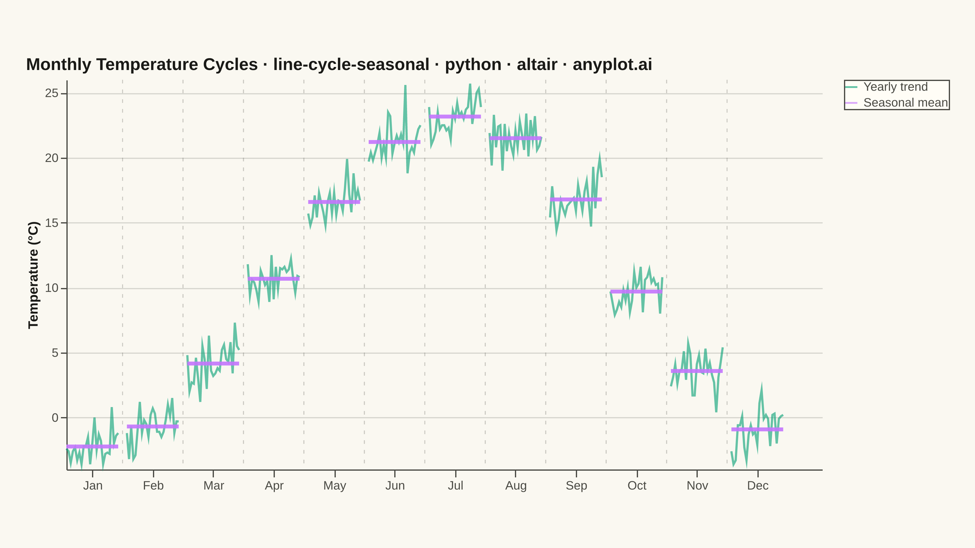
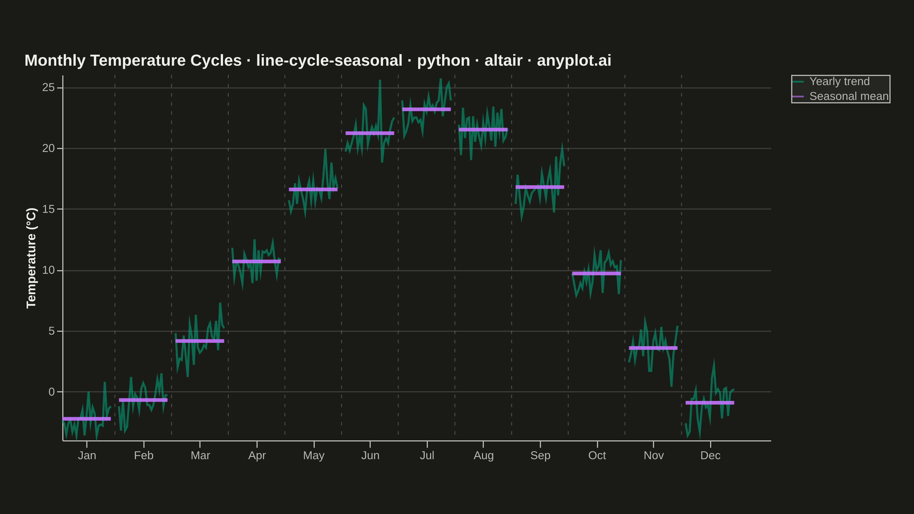
A cycle plot, also known as a seasonal subseries plot (introduced by William Cleveland), separates the seasonal pattern of a time series from the trend within each season. The series is split by seasonal period (e.g. one group per month or weekday); within each group the values are drawn in chronological order as a small line, and a horizontal reference line marks that group's mean. Comparing the mean lines across groups reveals the seasonal effect, while the slope of each subseries reveals the trend within that season — two patterns that are entangled in a standard time series plot.
""" anyplot.ai
line-cycle-seasonal: Cycle Plot (Seasonal Subseries)
Library: altair 6.2.1 | Python 3.13.13
Quality: 83/100 | Created: 2026-06-15
"""

import os
import sys

import numpy as np
import pandas as pd
from PIL import Image


# Remove current directory from sys.path to avoid local altair.py shadowing the package
script_dir = os.path.dirname(os.path.abspath(__file__))
sys.path = [p for p in sys.path if p != script_dir and os.path.abspath(p) != script_dir]

import altair as alt


# Theme tokens — Imprint palette, theme-adaptive chrome
THEME = os.getenv("ANYPLOT_THEME", "light")
PAGE_BG = "#FAF8F1" if THEME == "light" else "#1A1A17"
ELEVATED_BG = "#FFFDF6" if THEME == "light" else "#242420"
INK = "#1A1A17" if THEME == "light" else "#F0EFE8"
INK_SOFT = "#4A4A44" if THEME == "light" else "#B8B7B0"
INK_MUTED = "#6B6A63" if THEME == "light" else "#A8A79F"

IMPRINT_PALETTE = ["#009E73", "#C475FD", "#4467A3", "#BD8233", "#AE3030", "#2ABCCD", "#954477", "#99B314"]
BRAND = IMPRINT_PALETTE[0]  # always first series

# Data: monthly average temperatures, 25 years (1999–2023)
np.random.seed(42)
MONTHS = ["Jan", "Feb", "Mar", "Apr", "May", "Jun", "Jul", "Aug", "Sep", "Oct", "Nov", "Dec"]
N_MONTHS = 12
N_YEARS = 25
STRIDE = N_YEARS + 3  # 28 positions per month group (25 data + 3 gap)

# Northern-hemisphere seasonal baseline (°C) with a long-term warming trend
seasonal_base = np.array([-3.0, -1.0, 4.0, 10.0, 16.0, 20.0, 22.0, 21.0, 16.0, 9.0, 3.0, -2.0])

records = []
for y_idx in range(N_YEARS):
    for m_idx, month in enumerate(MONTHS):
        temp = seasonal_base[m_idx] + 0.06 * y_idx + np.random.normal(0, 1.2)
        records.append(
            {
                "month": month,
                "month_idx": m_idx,
                "year": 1999 + y_idx,
                "year_idx": y_idx,
                "temperature": round(temp, 1),
                "x_pos": m_idx * STRIDE + y_idx,
            }
        )

df = pd.DataFrame(records)

# Monthly means for horizontal reference lines
means = df.groupby(["month", "month_idx"])["temperature"].mean().reset_index()
means.columns = ["month", "month_idx", "mean_temp"]
means["x_start"] = means["month_idx"] * STRIDE
means["x_end"] = means["month_idx"] * STRIDE + N_YEARS - 1

# Series labels for shared legend
df["series"] = "Yearly trend"
means["series"] = "Seasonal mean"
SERIES_SCALE = alt.Scale(domain=["Yearly trend", "Seasonal mean"], range=[BRAND, IMPRINT_PALETTE[1]])

# Vertical dividers between month groups (centred in each gap)
dividers_df = pd.DataFrame({"x": [i * STRIDE + N_YEARS + 1 for i in range(N_MONTHS - 1)]})

# Title with length-scaled fontsize (baseline default = 16px at 67 chars)
title_text = "Monthly Temperature Cycles · line-cycle-seasonal · python · altair · anyplot.ai"
title_fs = max(11, round(16 * 67 / len(title_text))) if len(title_text) > 67 else 16

# X-axis: custom tick positions at the centre of each month group
x_ticks = [i * STRIDE + (N_YEARS - 1) / 2.0 for i in range(N_MONTHS)]
month_label_expr = (
    f"['Jan','Feb','Mar','Apr','May','Jun','Jul','Aug','Sep','Oct','Nov','Dec'][floor(datum.value / {STRIDE})]"
)

# Layer 1 — within-month chronological trend lines
lines = (
    alt.Chart(df)
    .mark_line(strokeWidth=1.8, opacity=0.60)
    .encode(
        x=alt.X(
            "x_pos:Q",
            title=None,
            axis=alt.Axis(values=x_ticks, labelExpr=month_label_expr, labelFontSize=10, gridOpacity=0, tickSize=6),
        ),
        y=alt.Y("temperature:Q", title="Temperature (°C)"),
        detail="month:N",
        color=alt.Color("series:N", scale=SERIES_SCALE, legend=alt.Legend(title=None)),
    )
)

# Layer 2 — monthly mean reference lines (key seasonal comparison signal)
mean_rules = (
    alt.Chart(means)
    .mark_rule(strokeWidth=3.2, opacity=0.9)
    .encode(
        x="x_start:Q",
        x2="x_end:Q",
        y="mean_temp:Q",
        color=alt.Color("series:N", scale=SERIES_SCALE, legend=alt.Legend(title=None)),
    )
)

# Layer 3 — subtle vertical dividers between month groups
dividers = (
    alt.Chart(dividers_df).mark_rule(color=INK_MUTED, strokeWidth=0.8, opacity=0.35, strokeDash=[3, 5]).encode(x="x:Q")
)

# Compose and configure
chart = (
    (lines + mean_rules + dividers)
    .properties(width=620, height=320, background=PAGE_BG, title=title_text)
    .configure_view(fill=PAGE_BG, stroke=None)
    .configure_title(fontSize=title_fs, color=INK, anchor="start")
    .configure_axis(
        domainColor=INK_SOFT, tickColor=INK_SOFT, labelColor=INK_SOFT, titleColor=INK, gridColor=INK, gridOpacity=0.15
    )
    .configure_legend(fillColor=ELEVATED_BG, strokeColor=INK_SOFT, labelColor=INK_SOFT, titleColor=INK)
)

# Save PNG + HTML (interactive)
TW, TH = 3200, 1800
chart.save(f"plot-{THEME}.png", scale_factor=4.0)
chart.save(f"plot-{THEME}.html")

# Pad PNG to exact canvas target (3200 × 1800)
_img = Image.open(f"plot-{THEME}.png").convert("RGB")
_w, _h = _img.size
if _w > TW or _h > TH:
    raise SystemExit(
        f"altair vl-convert produced {_w}×{_h}, exceeds target {TW}×{TH}. "
        f"Shrink chart .properties(width=, height=) and re-render."
    )
if _w < TW or _h < TH:
    _canvas = Image.new("RGB", (TW, TH), PAGE_BG)
    _canvas.paste(_img, ((TW - _w) // 2, (TH - _h) // 2))
    _canvas.save(f"plot-{THEME}.png")
Runnable source as JSON, for any HTTP client: https://api.anyplot.ai/specs/line-cycle-seasonal/altair/code. Any spec id and library id listed in llms-full.txt fit the same URL shape; every URL below is complete and callable.
{
  "spec_id": "line-cycle-seasonal",
  "language": "python",
  "library": "altair",
  "page": "https://anyplot.ai/line-cycle-seasonal/python/altair",
  "hub": "https://anyplot.ai/line-cycle-seasonal",
  "code_json": "https://api.anyplot.ai/specs/line-cycle-seasonal/altair/code",
  "spec_json": "https://api.anyplot.ai/specs/line-cycle-seasonal",
  "render_light_png": "https://storage.googleapis.com/anyplot-images/plots/line-cycle-seasonal/python/altair/plot-light.png",
  "render_dark_png": "https://storage.googleapis.com/anyplot-images/plots/line-cycle-seasonal/python/altair/plot-dark.png",
  "interactive_light_html": "https://storage.googleapis.com/anyplot-images/plots/line-cycle-seasonal/python/altair/plot-light.html",
  "interactive_dark_html": "https://storage.googleapis.com/anyplot-images/plots/line-cycle-seasonal/python/altair/plot-dark.html",
  "quality_score": 83.0,
  "license": "MIT",
  "guide": "https://anyplot.ai/llms.txt"
}
Part of Cycle Plot (Seasonal Subseries) on anyplot.ai.