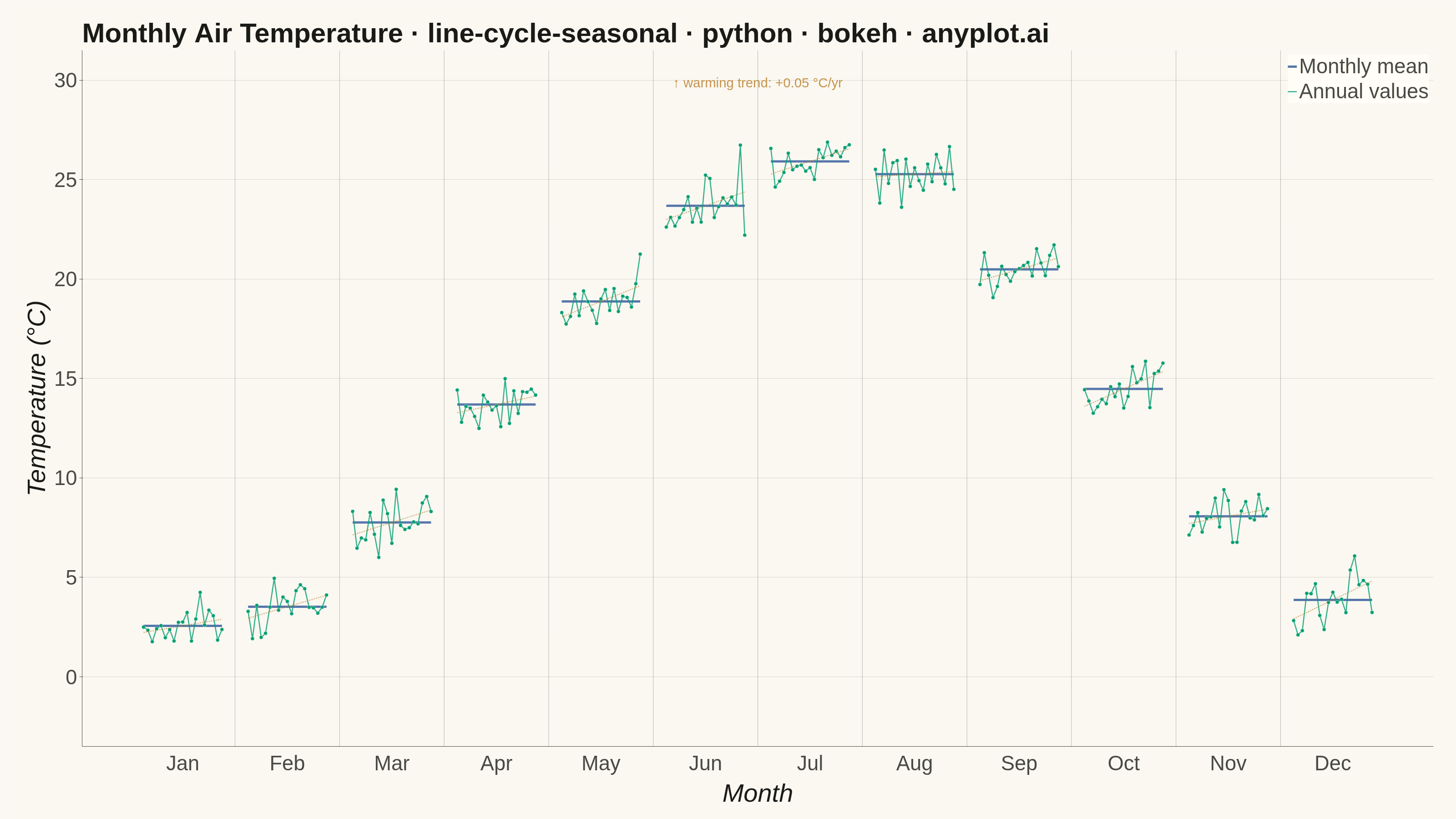
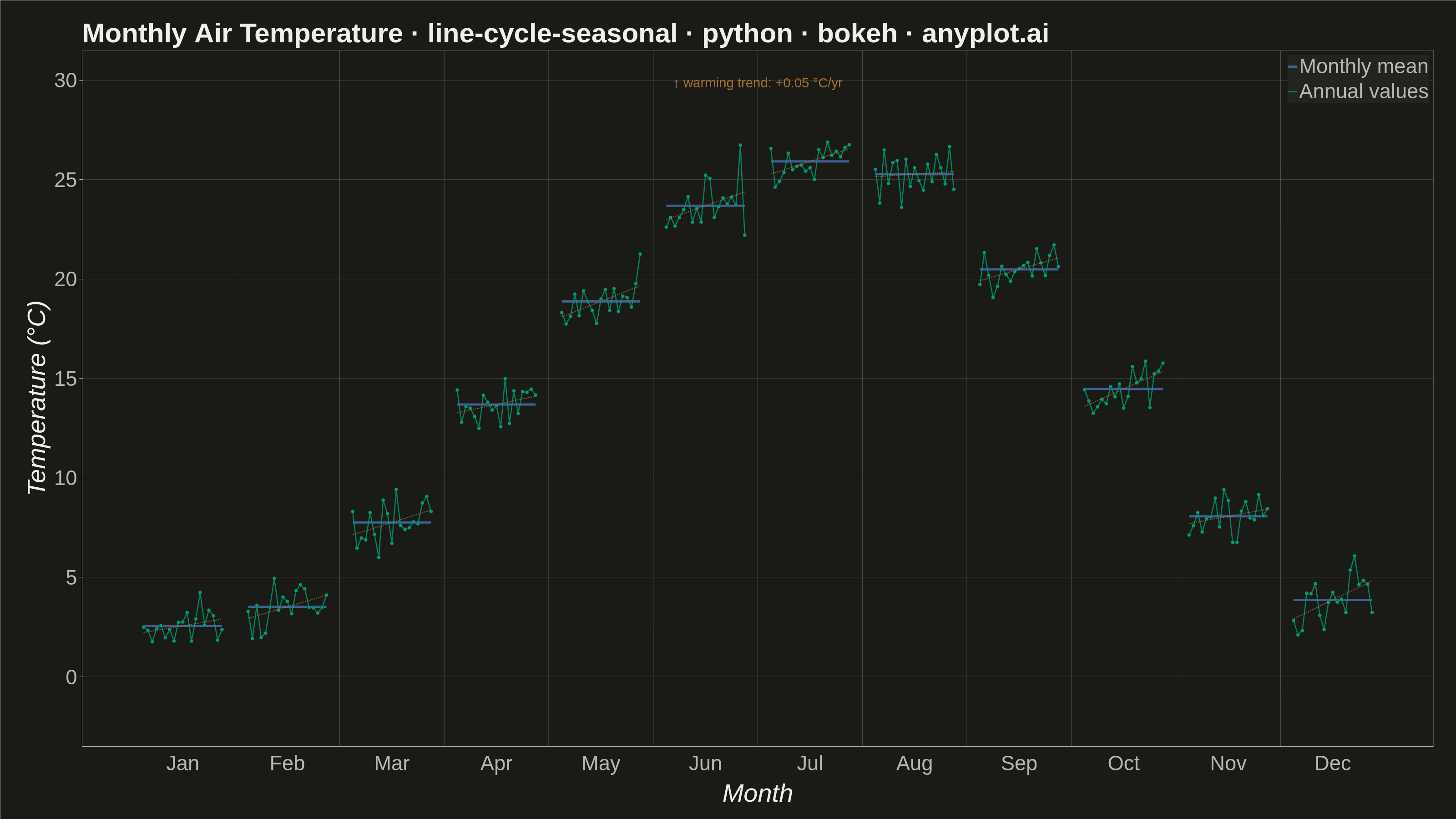
A cycle plot, also known as a seasonal subseries plot (introduced by William Cleveland), separates the seasonal pattern of a time series from the trend within each season. The series is split by seasonal period (e.g. one group per month or weekday); within each group the values are drawn in chronological order as a small line, and a horizontal reference line marks that group's mean. Comparing the mean lines across groups reveals the seasonal effect, while the slope of each subseries reveals the trend within that season — two patterns that are entangled in a standard time series plot.
""" anyplot.ai
line-cycle-seasonal: Cycle Plot (Seasonal Subseries)
Library: bokeh 3.9.1 | Python 3.13.13
Quality: 85/100 | Created: 2026-06-15
"""

import io
import os
import sys
import time
from pathlib import Path


# Workaround: remove the script's own directory from sys.path so that the file
# bokeh.py doesn't shadow the installed bokeh package on import.
original_path = sys.path.copy()
sys.path = [p for p in sys.path if p != "" and not (os.path.isfile(os.path.join(p, "bokeh.py")) if p else False)]

try:
    import numpy as np
    import pandas as pd
    from bokeh.io import output_file, save
    from bokeh.models import CustomJSTickFormatter, FixedTicker, Label
    from bokeh.plotting import figure
    from PIL import Image
    from selenium import webdriver
    from selenium.webdriver.chrome.options import Options
finally:
    sys.path = original_path

# Theme tokens
THEME = os.getenv("ANYPLOT_THEME", "light")
PAGE_BG = "#FAF8F1" if THEME == "light" else "#1A1A17"
ELEVATED_BG = "#FFFDF6" if THEME == "light" else "#242420"
INK = "#1A1A17" if THEME == "light" else "#F0EFE8"
INK_SOFT = "#4A4A44" if THEME == "light" else "#B8B7B0"

IMPRINT_PALETTE = ["#009E73", "#C475FD", "#4467A3", "#BD8233", "#AE3030", "#2ABCCD", "#954477", "#99B314"]
BRAND = IMPRINT_PALETTE[0]  # #009E73 — annual subseries lines (first series)
BLUE = IMPRINT_PALETTE[2]  # #4467A3 — seasonal mean reference lines

# Data: synthetic monthly average temperature (°C) at a mid-latitude station, 2005–2023
np.random.seed(42)
n_years = 19
months = ["Jan", "Feb", "Mar", "Apr", "May", "Jun", "Jul", "Aug", "Sep", "Oct", "Nov", "Dec"]
n_months = 12

seasonal_base = np.array([2.1, 3.4, 7.8, 13.2, 18.5, 22.8, 25.3, 24.9, 20.1, 14.0, 7.5, 3.2])
warming_rate = 0.05  # °C per year — long-term warming signal

rows = []
for yi in range(n_years):
    for mi in range(n_months):
        temp = seasonal_base[mi] + warming_rate * yi + np.random.normal(0, 0.8)
        rows.append({"year_idx": yi, "month_idx": mi, "temp": temp})
df = pd.DataFrame(rows)

# Layout: 19 data points per group (year_idx 0..18); gap=5; step=24
# → integer midpoints at 9, 33, 57, 81, ... for clean tick alignment
group_width = n_years - 1  # 18 (positions 0 to 18)
group_gap = 5
total_step = group_width + group_gap + 1  # 24

group_starts = [mi * total_step for mi in range(n_months)]
group_ends = [gs + group_width for gs in group_starts]
group_mids = [gs + group_width // 2 for gs in group_starts]  # 9, 33, 57, ...
group_means = [df[df["month_idx"] == mi]["temp"].mean() for mi in range(n_months)]

# Multi-line data for subseries (annual trend within each month group)
sub_xs = []
sub_ys = []
for mi in range(n_months):
    m_df = df[df["month_idx"] == mi].sort_values("year_idx")
    sub_xs.append([mi * total_step + int(yi) for yi in m_df["year_idx"]])
    sub_ys.append(m_df["temp"].tolist())

# Multi-line data for mean reference lines (horizontal span per group)
mean_xs = [[group_starts[mi], group_ends[mi]] for mi in range(n_months)]
mean_ys = [[group_means[mi], group_means[mi]] for mi in range(n_months)]

# Vertical divider positions (midpoint of each gap between groups)
div_xs = [[group_ends[mi] + (group_gap + 1) / 2.0] * 2 for mi in range(n_months - 1)]
div_ys = [[-3.5, 31.5] for _ in range(n_months - 1)]

# Scatter markers — flattened positions for all annual data points
all_x = [x for xs in sub_xs for x in xs]
all_y = [y for ys in sub_ys for y in ys]

# Linear trend per monthly group to show within-season warming signal
trend_xs = []
trend_ys = []
for mi in range(n_months):
    m_x = np.array(sub_xs[mi], dtype=float)
    m_y = np.array(sub_ys[mi], dtype=float)
    coeffs = np.polyfit(m_x, m_y, 1)
    trend_xs.append([float(m_x[0]), float(m_x[-1])])
    trend_ys.append([float(coeffs[0] * m_x[0] + coeffs[1]), float(coeffs[0] * m_x[-1] + coeffs[1])])

# Title — scale fontsize for long title
title_str = "Monthly Air Temperature · line-cycle-seasonal · python · bokeh · anyplot.ai"
n_chars = len(title_str)
title_fontsize = max(34, round(50 * 67 / n_chars)) if n_chars > 67 else 50

# Build figure
p = figure(
    width=3200,
    height=1800,
    title=title_str,
    x_axis_label="Month",
    y_axis_label="Temperature (°C)",
    toolbar_location=None,
    min_border_bottom=160,
    min_border_left=180,
    min_border_top=110,
    min_border_right=50,
    y_range=(-3.5, 31.5),
)

# Group dividers (drawn first, renders below data)
p.multi_line(div_xs, div_ys, line_color=INK_SOFT, line_alpha=0.38, line_width=1)

# Seasonal mean reference lines (thick blue, drawn below annual lines)
p.multi_line(mean_xs, mean_ys, line_color=BLUE, line_width=5, line_alpha=0.9, legend_label="Monthly mean")

# Annual subseries lines (brand green, one per month group)
p.multi_line(sub_xs, sub_ys, line_color=BRAND, line_width=2.5, line_alpha=0.8, legend_label="Annual values")

# Scatter markers for individual annual data points
p.scatter(all_x, all_y, size=8, color=BRAND, line_color=PAGE_BG, line_width=0.5)

# Dashed trend lines per group — make the within-season warming signal explicit
AMBER = IMPRINT_PALETTE[3]  # #BD8233 — trend annotation distinct from data colors
p.multi_line(trend_xs, trend_ys, line_color=AMBER, line_width=2.0, line_alpha=0.65, line_dash="dashed")
center_x = (group_starts[0] + group_ends[-1]) / 2.0
warming_label = Label(
    x=center_x,
    y=29.5,
    text="↑ warming trend: +0.05 °C/yr",
    text_font_size="22pt",
    text_color=AMBER,
    text_align="center",
    text_alpha=0.85,
    background_fill_alpha=0.0,
    border_line_alpha=0.0,
)
p.add_layout(warming_label)

# Custom x-axis: ticks at integer group midpoints mapped to month names
js_labels = "{" + ", ".join(f'"{mid}": "{m}"' for mid, m in zip(group_mids, months, strict=True)) + "}"
p.xaxis.ticker = FixedTicker(ticks=group_mids)
p.xaxis.formatter = CustomJSTickFormatter(
    code=(f"const labels = {js_labels}; return labels[String(Math.round(tick))] || '';")
)
p.xaxis.major_tick_line_color = None
p.xaxis.minor_tick_line_color = None

# Grid
p.xgrid.grid_line_color = None
p.ygrid.grid_line_color = INK
p.ygrid.grid_line_alpha = 0.15

# Remove full-box outline; axis lines provide the L-shaped spine
p.outline_line_color = None
p.xaxis.axis_line_color = INK_SOFT
p.yaxis.axis_line_color = INK_SOFT
p.yaxis.major_tick_line_color = INK_SOFT
p.yaxis.minor_tick_line_color = None

# Theme-adaptive chrome
p.background_fill_color = PAGE_BG
p.border_fill_color = PAGE_BG

p.title.text_font_size = f"{title_fontsize}pt"
p.title.text_color = INK
p.title.text_font_style = "bold"

p.xaxis.axis_label_text_font_size = "42pt"
p.yaxis.axis_label_text_font_size = "42pt"
p.xaxis.axis_label_text_color = INK
p.yaxis.axis_label_text_color = INK

p.xaxis.major_label_text_font_size = "34pt"
p.yaxis.major_label_text_font_size = "34pt"
p.xaxis.major_label_text_color = INK_SOFT
p.yaxis.major_label_text_color = INK_SOFT

# Legend
p.legend.background_fill_color = ELEVATED_BG
p.legend.border_line_color = None
p.legend.label_text_color = INK_SOFT
p.legend.label_text_font_size = "34pt"
p.legend.location = "top_right"

# Save interactive HTML
output_file(f"plot-{THEME}.html")
save(p)

# Screenshot with headless Chrome (Selenium 4 / Selenium Manager).
# Chrome's internal overhead shrinks the viewport below --window-size by ~139 px;
# use H + 200 buffer, then crop to exact canvas dimensions with PIL.
W, H = 3200, 1800
opts = Options()
for arg in (
    "--headless=new",
    "--no-sandbox",
    "--disable-dev-shm-usage",
    "--disable-gpu",
    f"--window-size={W},{H + 200}",
    "--hide-scrollbars",
    "--force-device-scale-factor=1",
):
    opts.add_argument(arg)
driver = webdriver.Chrome(options=opts)
driver.set_window_size(W, H + 200)
driver.get(f"file://{Path(f'plot-{THEME}.html').resolve()}")
time.sleep(3)
raw = driver.get_screenshot_as_png()
driver.quit()
Image.open(io.BytesIO(raw)).crop((0, 0, W, H)).save(f"plot-{THEME}.png")
Runnable source as JSON, for any HTTP client: https://api.anyplot.ai/specs/line-cycle-seasonal/bokeh/code. Any spec id and library id listed in llms-full.txt fit the same URL shape; every URL below is complete and callable.
{
  "spec_id": "line-cycle-seasonal",
  "language": "python",
  "library": "bokeh",
  "page": "https://anyplot.ai/line-cycle-seasonal/python/bokeh",
  "hub": "https://anyplot.ai/line-cycle-seasonal",
  "code_json": "https://api.anyplot.ai/specs/line-cycle-seasonal/bokeh/code",
  "spec_json": "https://api.anyplot.ai/specs/line-cycle-seasonal",
  "render_light_png": "https://storage.googleapis.com/anyplot-images/plots/line-cycle-seasonal/python/bokeh/plot-light.png",
  "render_dark_png": "https://storage.googleapis.com/anyplot-images/plots/line-cycle-seasonal/python/bokeh/plot-dark.png",
  "interactive_light_html": "https://storage.googleapis.com/anyplot-images/plots/line-cycle-seasonal/python/bokeh/plot-light.html",
  "interactive_dark_html": "https://storage.googleapis.com/anyplot-images/plots/line-cycle-seasonal/python/bokeh/plot-dark.html",
  "quality_score": 85.0,
  "license": "MIT",
  "guide": "https://anyplot.ai/llms.txt"
}
Part of Cycle Plot (Seasonal Subseries) on anyplot.ai.