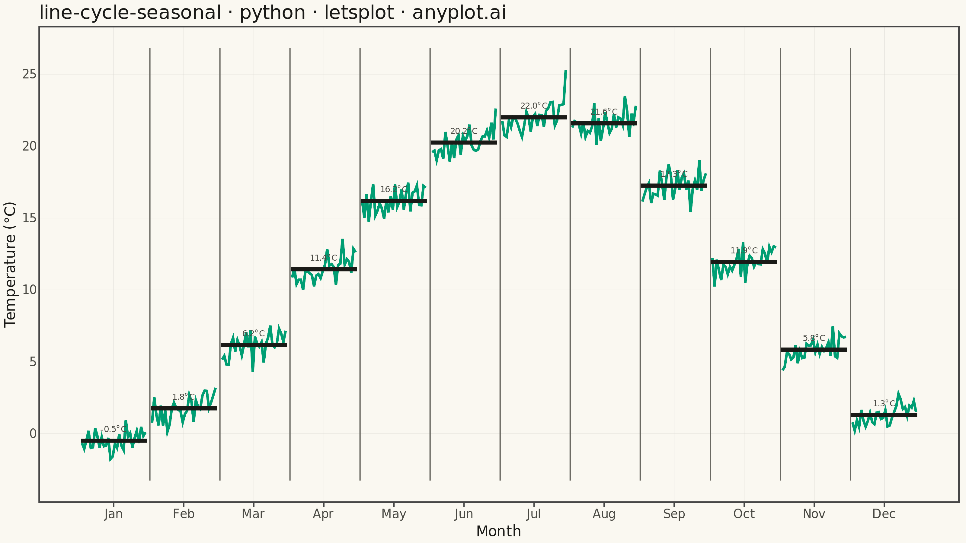
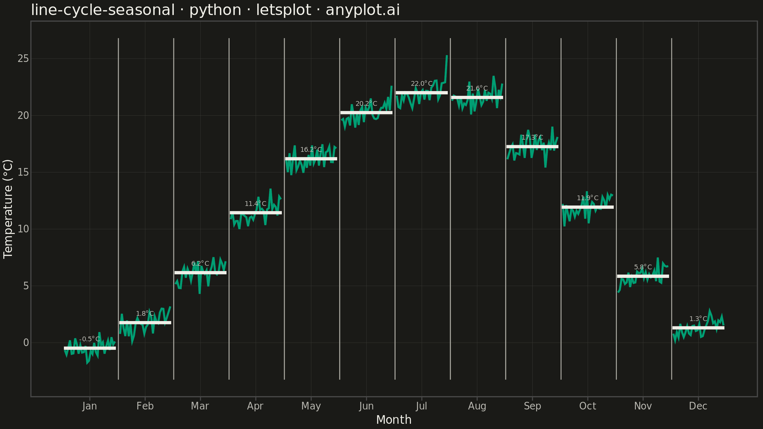
A cycle plot, also known as a seasonal subseries plot (introduced by William Cleveland), separates the seasonal pattern of a time series from the trend within each season. The series is split by seasonal period (e.g. one group per month or weekday); within each group the values are drawn in chronological order as a small line, and a horizontal reference line marks that group's mean. Comparing the mean lines across groups reveals the seasonal effect, while the slope of each subseries reveals the trend within that season — two patterns that are entangled in a standard time series plot.
""" anyplot.ai
line-cycle-seasonal: Cycle Plot (Seasonal Subseries)
Library: letsplot 4.10.1 | Python 3.13.13
Quality: 86/100 | Created: 2026-06-15
"""

import os

import numpy as np
import pandas as pd
from lets_plot import (
    LetsPlot,
    aes,
    element_blank,
    element_line,
    element_rect,
    element_text,
    geom_line,
    geom_segment,
    geom_text,
    ggplot,
    ggsize,
    labs,
    scale_x_continuous,
    theme,
)
from lets_plot.export import ggsave


LetsPlot.setup_html()

# Theme tokens
THEME = os.getenv("ANYPLOT_THEME", "light")
PAGE_BG = "#FAF8F1" if THEME == "light" else "#1A1A17"
ELEVATED_BG = "#FFFDF6" if THEME == "light" else "#242420"
INK = "#1A1A17" if THEME == "light" else "#F0EFE8"
INK_SOFT = "#4A4A44" if THEME == "light" else "#B8B7B0"
INK_MUTED = "#6B6A63" if THEME == "light" else "#A8A79F"
GRID_LINE = "#D8D6D0" if THEME == "light" else "#3A3A36"

BRAND = "#009E73"  # Imprint palette position 1 — always first series

# Data: monthly mean temperature (°C) for a temperate European city, 1991–2020
np.random.seed(42)
years = np.arange(1991, 2021)  # 30 years
month_names = ["Jan", "Feb", "Mar", "Apr", "May", "Jun", "Jul", "Aug", "Sep", "Oct", "Nov", "Dec"]

# Seasonal baseline + gentle warming trend (0.045 °C/year → ~1.3 °C over 30 years)
seasonal_base = np.array([-1.0, 1.2, 5.5, 10.8, 15.6, 19.4, 21.3, 20.9, 16.7, 11.2, 5.0, 0.8])
warming = 0.045

records = []
for m_idx in range(12):
    for y_idx, year in enumerate(years):
        temp = seasonal_base[m_idx] + warming * y_idx + np.random.normal(0, 0.7)
        records.append(
            {
                "month_num": m_idx + 1,
                "month": month_names[m_idx],
                "year": year,
                "y_idx": y_idx,
                "temperature": round(temp, 2),
            }
        )

df = pd.DataFrame(records)

# x-positions: each month group occupies GROUP_WIDTH units (30 pts + 2-unit gap)
GROUP_WIDTH = 32
df["x_pos"] = (df["month_num"] - 1) * GROUP_WIDTH + df["y_idx"]

# Per-month mean reference line endpoints
means = df.groupby("month_num")["temperature"].mean().reset_index()
means["x_start"] = (means["month_num"] - 1) * GROUP_WIDTH - 0.5
means["x_end"] = means["x_start"] + 30.0
means["x_center"] = (means["month_num"] - 1) * GROUP_WIDTH + 14.5
means["label"] = means["temperature"].round(1).astype(str) + "°C"
means["label_y"] = means["temperature"] + 0.8

# Subtle vertical dividers between month groups
divider_xs = [(m * GROUP_WIDTH - 1.0) for m in range(1, 12)]
y_lo = df["temperature"].min() - 1.5
y_hi = df["temperature"].max() + 1.5
dividers = pd.DataFrame({"x": divider_xs, "xend": divider_xs, "y": [y_lo] * 11, "yend": [y_hi] * 11})

# X-axis tick at center of each month group
tick_breaks = [(m - 1) * GROUP_WIDTH + 14.5 for m in range(1, 13)]

title = "line-cycle-seasonal · python · letsplot · anyplot.ai"
# 52 chars < 67 baseline → title_size stays at default 16
title_size = 16

anyplot_theme = theme(
    plot_background=element_rect(fill=PAGE_BG, color=PAGE_BG),
    panel_background=element_rect(fill=PAGE_BG),
    panel_border=element_blank(),
    panel_grid_major=element_line(color=GRID_LINE, size=0.25),
    panel_grid_minor=element_blank(),
    axis_title=element_text(color=INK, size=12),
    axis_text=element_text(color=INK_SOFT, size=10),
    axis_line=element_line(color=INK_SOFT),
    plot_title=element_text(color=INK, size=title_size),
    legend_position="none",
)

plot = (
    ggplot()
    # Subtle vertical dividers between month groups
    + geom_segment(data=dividers, mapping=aes(x="x", xend="xend", y="y", yend="yend"), color=INK_MUTED, size=0.4)
    # Subseries: chronological line per month
    + geom_line(data=df, mapping=aes(x="x_pos", y="temperature", group="month_num"), color=BRAND, size=0.9)
    # Seasonal mean reference lines (key visual for comparing seasons)
    + geom_segment(
        data=means, mapping=aes(x="x_start", xend="x_end", y="temperature", yend="temperature"), color=INK, size=1.5
    )
    # Mean temperature annotations — letsplot geom_text labels each season's average
    + geom_text(
        data=means,
        mapping=aes(x="x_center", y="label_y", label="label"),
        color=INK_SOFT,
        size=3.5,
        vjust=0.5,
        hjust=0.5,
    )
    + scale_x_continuous(breaks=tick_breaks, labels=month_names)
    + labs(x="Month", y="Temperature (°C)", title=title)
    + anyplot_theme
    + ggsize(800, 450)
)

ggsave(plot, f"plot-{THEME}.png", path=".", scale=4)
ggsave(plot, f"plot-{THEME}.html", path=".")
Runnable source as JSON, for any HTTP client: https://api.anyplot.ai/specs/line-cycle-seasonal/letsplot/code. Any spec id and library id listed in llms-full.txt fit the same URL shape; every URL below is complete and callable.
{
  "spec_id": "line-cycle-seasonal",
  "language": "python",
  "library": "letsplot",
  "page": "https://anyplot.ai/line-cycle-seasonal/python/letsplot",
  "hub": "https://anyplot.ai/line-cycle-seasonal",
  "code_json": "https://api.anyplot.ai/specs/line-cycle-seasonal/letsplot/code",
  "spec_json": "https://api.anyplot.ai/specs/line-cycle-seasonal",
  "render_light_png": "https://storage.googleapis.com/anyplot-images/plots/line-cycle-seasonal/python/letsplot/plot-light.png",
  "render_dark_png": "https://storage.googleapis.com/anyplot-images/plots/line-cycle-seasonal/python/letsplot/plot-dark.png",
  "interactive_light_html": "https://storage.googleapis.com/anyplot-images/plots/line-cycle-seasonal/python/letsplot/plot-light.html",
  "interactive_dark_html": "https://storage.googleapis.com/anyplot-images/plots/line-cycle-seasonal/python/letsplot/plot-dark.html",
  "quality_score": 86.0,
  "license": "MIT",
  "guide": "https://anyplot.ai/llms.txt"
}
Part of Cycle Plot (Seasonal Subseries) on anyplot.ai.