The same plot in 14 other libraries — JavaScript: Chart.js, Apache ECharts, Highcharts, MUI X Charts; Python: Altair, Bokeh, lets-plot, Matplotlib, Plotly, plotnine, Pygal, Seaborn; R: ggplot2; Julia: Makie.jl. Compare all 15 side by side: Logistic Regression Curve Plot in Python, R, Julia and JavaScript.
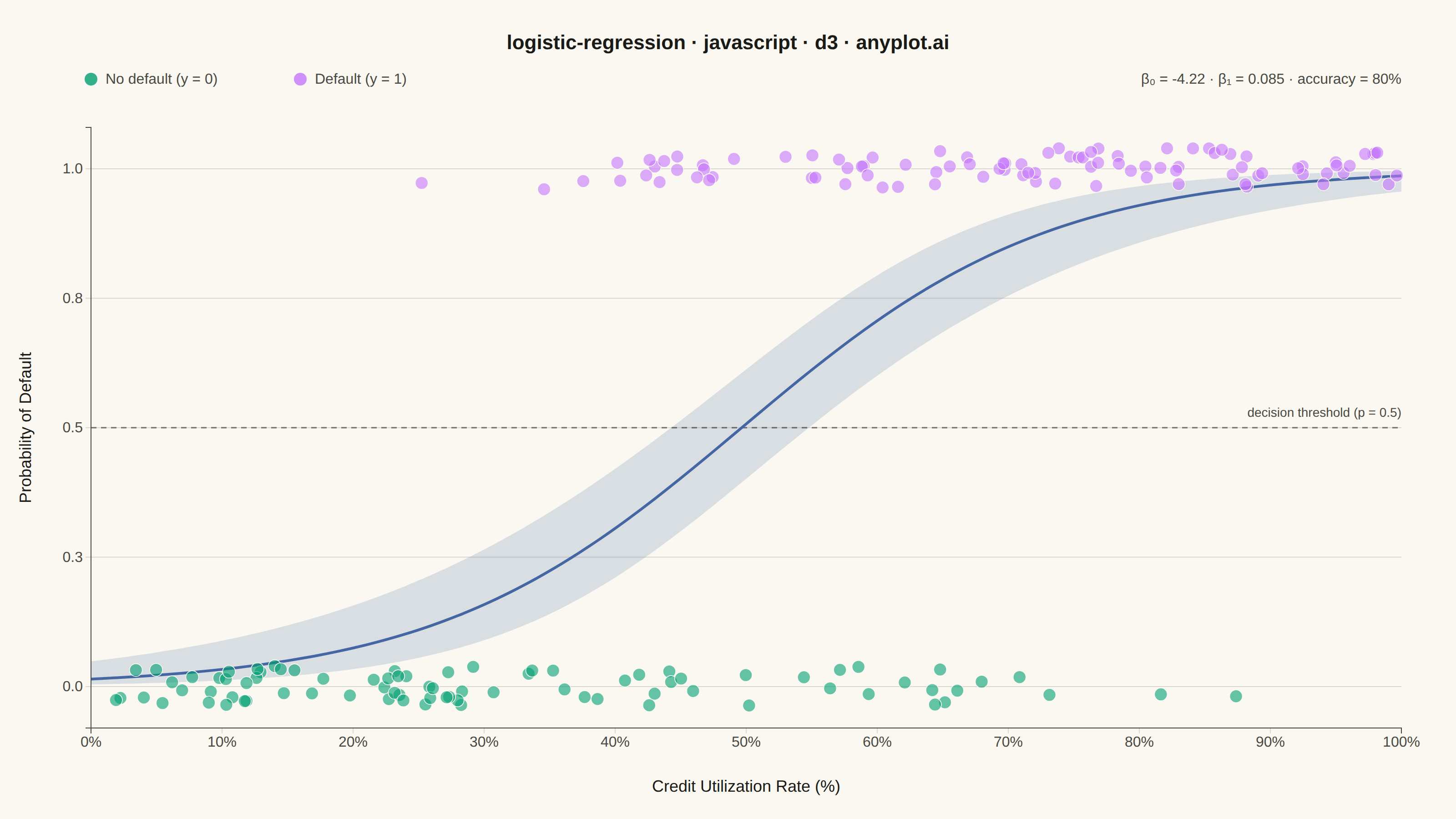
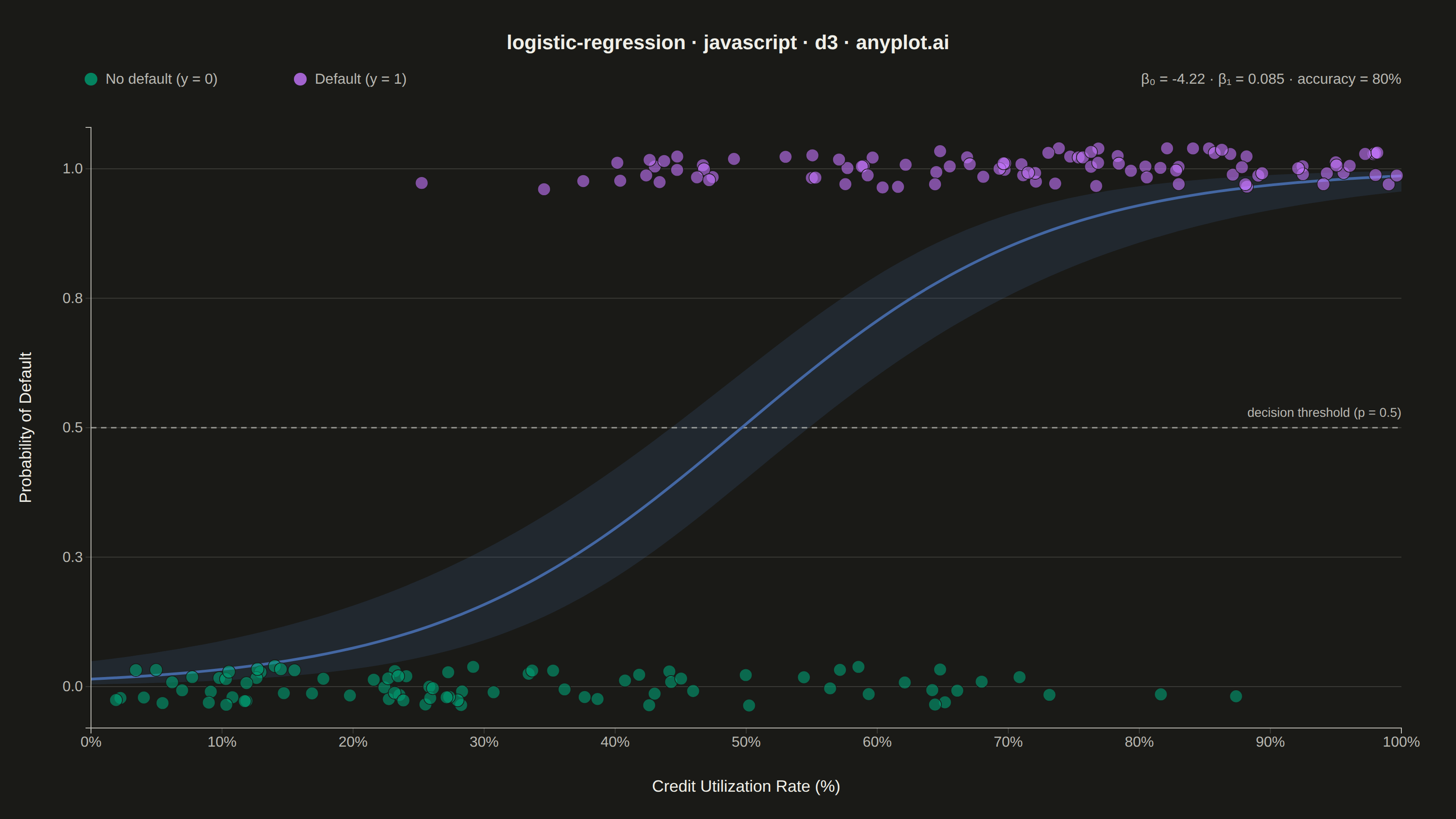
A logistic regression visualization showing the characteristic S-shaped (sigmoid) probability curve for binary classification. The plot displays data points colored by their binary class, the fitted logistic curve representing predicted probabilities, confidence intervals around the curve, and a dashed decision threshold line at probability 0.5. This visualization is essential for understanding how a logistic model maps continuous input features to class probabilities.
// anyplot.ai
// logistic-regression: Logistic Regression Curve Plot
// Library: d3 7.9.0 | JavaScript 22.23.2
// Quality: 92/100 | Created: 2026-09-02

const t = window.ANYPLOT_TOKENS;
const { width, height } = window.ANYPLOT_SIZE;
const margin = { top: 140, right: 60, bottom: 100, left: 100 };
const iw = width - margin.left - margin.right;
const ih = height - margin.top - margin.bottom;

// --- Data: synthetic credit-risk scenario (deterministic LCG) --------------
let seed = 42;
function rand() {
  seed = (seed * 1664525 + 1013904223) % 4294967296;
  return seed / 4294967296;
}

const n = 180;
const beta0True = -4.2;
const beta1True = 0.085;

const points = [];
for (let i = 0; i < n; i++) {
  const utilization = rand() * 100;
  const logit = beta0True + beta1True * utilization;
  const pTrue = 1 / (1 + Math.exp(-logit));
  const defaulted = rand() < pTrue ? 1 : 0;
  points.push({ utilization, defaulted });
}

// --- Fit logistic regression via Newton-Raphson (IRLS) ----------------------
let b0 = 0;
let b1 = 0;
for (let iter = 0; iter < 20; iter++) {
  let g0 = 0;
  let g1 = 0;
  let h00 = 0;
  let h01 = 0;
  let h11 = 0;
  for (const d of points) {
    const eta = b0 + b1 * d.utilization;
    const p = 1 / (1 + Math.exp(-eta));
    const w = p * (1 - p);
    const err = d.defaulted - p;
    g0 += err;
    g1 += err * d.utilization;
    h00 += w;
    h01 += w * d.utilization;
    h11 += w * d.utilization * d.utilization;
  }
  const det = h00 * h11 - h01 * h01;
  b0 += (h11 * g0 - h01 * g1) / det;
  b1 += (h00 * g1 - h01 * g0) / det;
}

// Covariance matrix = inverse Fisher information at the MLE — feeds the 95% CI band.
let h00f = 0;
let h01f = 0;
let h11f = 0;
for (const d of points) {
  const eta = b0 + b1 * d.utilization;
  const p = 1 / (1 + Math.exp(-eta));
  const w = p * (1 - p);
  h00f += w;
  h01f += w * d.utilization;
  h11f += w * d.utilization * d.utilization;
}
const detF = h00f * h11f - h01f * h01f;
const cov00 = h11f / detF;
const cov01 = -h01f / detF;
const cov11 = h00f / detF;

const accuracy =
  points.filter((d) => {
    const predicted = 1 / (1 + Math.exp(-(b0 + b1 * d.utilization))) >= 0.5 ? 1 : 0;
    return predicted === d.defaulted;
  }).length / n;

// --- Fitted curve + 95% confidence band over a grid --------------------------
const gridN = 100;
const curve = [];
for (let i = 0; i <= gridN; i++) {
  const xi = (i / gridN) * 100;
  const eta = b0 + b1 * xi;
  const seEta = Math.sqrt(cov00 + 2 * xi * cov01 + xi * xi * cov11);
  curve.push({
    x: xi,
    p: 1 / (1 + Math.exp(-eta)),
    lo: 1 / (1 + Math.exp(-(eta - 1.96 * seEta))),
    hi: 1 / (1 + Math.exp(-(eta + 1.96 * seEta))),
  });
}

// Jitter for point display only — class assignment itself stays binary.
const jittered = points.map((d) => ({
  ...d,
  yJitter: d.defaulted + (rand() - 0.5) * 0.08,
}));

// --- Scales -------------------------------------------------------------------
const x = d3.scaleLinear().domain([0, 100]).range([0, iw]);
const y = d3.scaleLinear().domain([-0.08, 1.08]).range([ih, 0]);

// --- SVG mount ------------------------------------------------------------
const svg = d3.select("#container").append("svg").attr("width", width).attr("height", height);
const g = svg.append("g").attr("transform", `translate(${margin.left},${margin.top})`);

// --- Gridlines (y-axis only) -------------------------------------------------
g.append("g")
  .call(d3.axisLeft(y).tickValues([0, 0.25, 0.5, 0.75, 1]).tickSize(-iw).tickFormat(""))
  .call((gr) => gr.select(".domain").remove())
  .call((gr) => gr.selectAll("line").attr("stroke", t.grid));

// --- Confidence band ----------------------------------------------------------
const band = d3
  .area()
  .x((d) => x(d.x))
  .y0((d) => y(d.lo))
  .y1((d) => y(d.hi))
  .curve(d3.curveMonotoneX);
g.append("path").datum(curve).attr("d", band).attr("fill", t.palette[2]).attr("opacity", 0.18);

// --- Decision threshold line ---------------------------------------------------
g.append("line")
  .attr("x1", 0)
  .attr("x2", iw)
  .attr("y1", y(0.5))
  .attr("y2", y(0.5))
  .attr("stroke", t.ink)
  .attr("stroke-width", 1.5)
  .attr("stroke-dasharray", "6,5")
  .attr("opacity", 0.55);

g.append("text")
  .attr("x", iw)
  .attr("y", y(0.5) - 12)
  .attr("text-anchor", "end")
  .attr("fill", t.inkSoft)
  .style("font-size", "14px")
  .text("decision threshold (p = 0.5)");

// --- Fitted logistic curve ------------------------------------------------------
const line = d3
  .line()
  .x((d) => x(d.x))
  .y((d) => y(d.p))
  .curve(d3.curveMonotoneX);
g.append("path").datum(curve).attr("d", line).attr("fill", "none").attr("stroke", t.palette[2]).attr("stroke-width", 3);

// --- Data points (jittered, colored by class) -----------------------------------
g.selectAll("circle")
  .data(jittered)
  .join("circle")
  .attr("cx", (d) => x(d.utilization))
  .attr("cy", (d) => y(d.yJitter))
  .attr("r", 7)
  .attr("fill", (d) => (d.defaulted ? t.palette[1] : t.palette[0]))
  .attr("fill-opacity", 0.6)
  .attr("stroke", t.pageBg)
  .attr("stroke-width", 0.8);

// --- Axes -----------------------------------------------------------------------
const xAxis = g
  .append("g")
  .attr("transform", `translate(0,${ih})`)
  .call(d3.axisBottom(x).ticks(8).tickFormat((d) => `${d}%`));
const yAxis = g.append("g").call(d3.axisLeft(y).tickValues([0, 0.25, 0.5, 0.75, 1]));
for (const ax of [xAxis, yAxis]) {
  ax.selectAll("text").attr("fill", t.inkSoft).style("font-size", "16px");
  ax.selectAll("line").attr("stroke", t.grid);
  ax.select(".domain").attr("stroke", t.inkSoft);
}

// --- Axis labels ------------------------------------------------------------
g.append("text")
  .attr("x", iw / 2)
  .attr("y", ih + 70)
  .attr("text-anchor", "middle")
  .attr("fill", t.ink)
  .style("font-size", "18px")
  .text("Credit Utilization Rate (%)");

g.append("text")
  .attr("transform", "rotate(-90)")
  .attr("x", -ih / 2)
  .attr("y", -66)
  .attr("text-anchor", "middle")
  .attr("fill", t.ink)
  .style("font-size", "18px")
  .text("Probability of Default");

// --- Header row: legend + model stats (kept clear of the plot area) -------------
const legendData = [
  { label: "No default (y = 0)", color: t.palette[0] },
  { label: "Default (y = 1)", color: t.palette[1] },
];
const legendG = svg.append("g").attr("transform", `translate(${margin.left}, 92)`);
legendData.forEach((item, i) => {
  const row = legendG.append("g").attr("transform", `translate(${i * 230}, 0)`);
  row.append("circle").attr("r", 7).attr("cy", -5).attr("fill", item.color).attr("fill-opacity", 0.8);
  row.append("text").attr("x", 16).attr("fill", t.inkSoft).style("font-size", "16px").text(item.label);
});

svg
  .append("text")
  .attr("x", width - margin.right)
  .attr("y", 92)
  .attr("text-anchor", "end")
  .attr("fill", t.inkSoft)
  .style("font-size", "16px")
  .text(`β₀ = ${b0.toFixed(2)} · β₁ = ${b1.toFixed(3)} · accuracy = ${(accuracy * 100).toFixed(0)}%`);

// --- Title -----------------------------------------------------------------
svg
  .append("text")
  .attr("x", width / 2)
  .attr("y", 54)
  .attr("text-anchor", "middle")
  .attr("fill", t.ink)
  .style("font-size", "22px")
  .style("font-weight", "600")
  .text("logistic-regression · javascript · d3 · anyplot.ai");
Runnable source as JSON, for any HTTP client: https://api.anyplot.ai/specs/logistic-regression/d3/code. Any spec id and library id listed in llms-full.txt fit the same URL shape; every URL below is complete and callable.
{
  "spec_id": "logistic-regression",
  "language": "javascript",
  "library": "d3",
  "page": "https://anyplot.ai/logistic-regression/javascript/d3",
  "hub": "https://anyplot.ai/logistic-regression",
  "code_json": "https://api.anyplot.ai/specs/logistic-regression/d3/code",
  "spec_json": "https://api.anyplot.ai/specs/logistic-regression",
  "render_light_png": "https://storage.googleapis.com/anyplot-images/plots/logistic-regression/javascript/d3/plot-light.png",
  "render_dark_png": "https://storage.googleapis.com/anyplot-images/plots/logistic-regression/javascript/d3/plot-dark.png",
  "interactive_light_html": "https://storage.googleapis.com/anyplot-images/plots/logistic-regression/javascript/d3/plot-light.html",
  "interactive_dark_html": "https://storage.googleapis.com/anyplot-images/plots/logistic-regression/javascript/d3/plot-dark.html",
  "quality_score": 92.0,
  "license": "MIT",
  "guide": "https://anyplot.ai/llms.txt"
}
Part of Logistic Regression Curve Plot on anyplot.ai.