The same plot in 14 other libraries — JavaScript: Chart.js, D3.js, Apache ECharts, Highcharts; Python: Altair, Bokeh, lets-plot, Matplotlib, Plotly, plotnine, Pygal, Seaborn; R: ggplot2; Julia: Makie.jl. Compare all 15 side by side: Logistic Regression Curve Plot in Python, R, Julia and JavaScript.
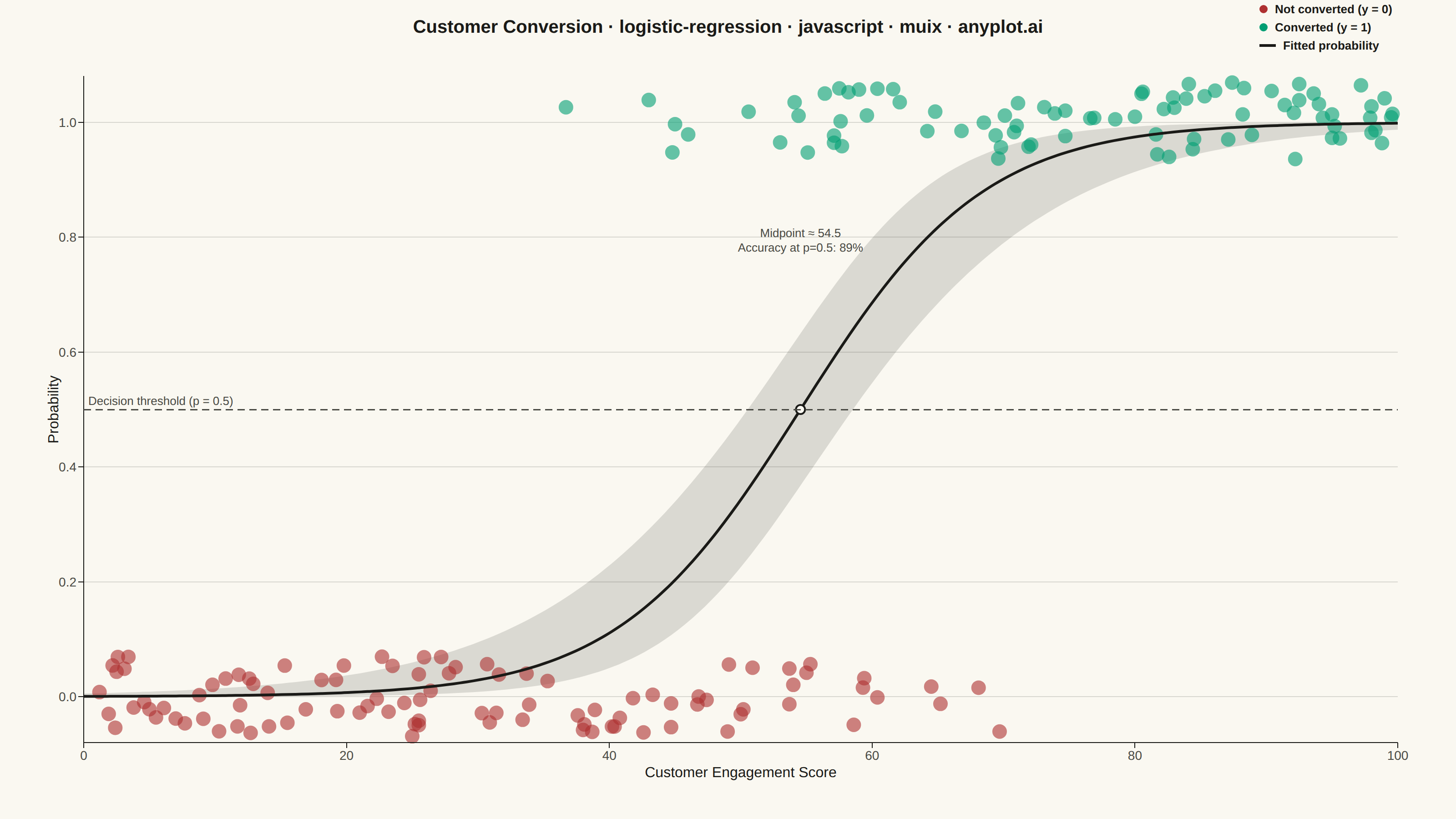
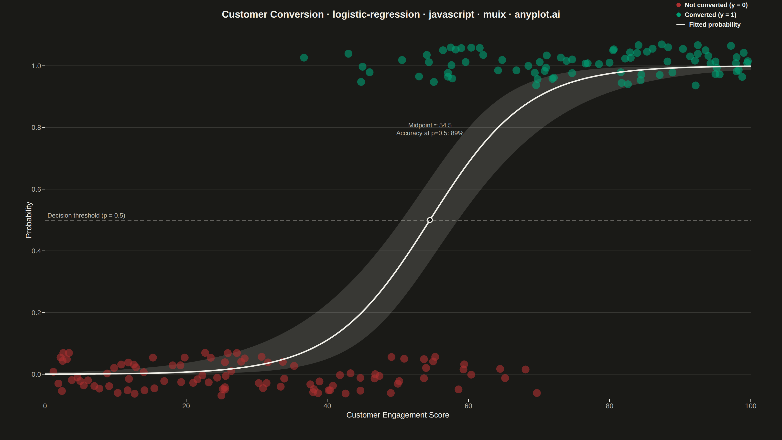
A logistic regression visualization showing the characteristic S-shaped (sigmoid) probability curve for binary classification. The plot displays data points colored by their binary class, the fitted logistic curve representing predicted probabilities, confidence intervals around the curve, and a dashed decision threshold line at probability 0.5. This visualization is essential for understanding how a logistic model maps continuous input features to class probabilities.
// anyplot.ai
// logistic-regression: Logistic Regression Curve Plot
// Library: muix 7.29.1 | JavaScript 22.23.2
// Quality: 92/100 | Created: 2026-09-02

import { ChartContainer } from "@mui/x-charts/ChartContainer";
import { LinePlot } from "@mui/x-charts/LineChart";
import { ScatterPlot } from "@mui/x-charts/ScatterChart";
import { ChartsXAxis } from "@mui/x-charts/ChartsXAxis";
import { ChartsYAxis } from "@mui/x-charts/ChartsYAxis";
import { ChartsGrid } from "@mui/x-charts/ChartsGrid";
import { ChartsReferenceLine } from "@mui/x-charts/ChartsReferenceLine";
import { useXScale, useYScale } from "@mui/x-charts/hooks";

const t = window.ANYPLOT_TOKENS;
const { width, height } = window.ANYPLOT_SIZE;

// Reproducible LCG (seed 42) — no Math.random() in the browser harness context
let seed = 42;
function rng() {
  seed = (1664525 * seed + 1013904223) >>> 0;
  return seed / 4294967296;
}

function hexToRgba(hex, alpha) {
  const r = parseInt(hex.slice(1, 3), 16);
  const g = parseInt(hex.slice(3, 5), 16);
  const b = parseInt(hex.slice(5, 7), 16);
  return `rgba(${r}, ${g}, ${b}, ${alpha})`;
}

// --- Data: marketing conversion vs. customer engagement score --------------
// True generating relationship — a customer with a higher engagement score
// (0-100) is more likely to convert, with a decision midpoint around 55.
function trueProbability(score) {
  return 1 / (1 + Math.exp(-(0.09 * (score - 55))));
}

const N_POINTS = 180;
const engagementScores = Array.from(
  { length: N_POINTS },
  () => Math.round(rng() * 1000) / 10,
);
const converted = engagementScores.map((score) => (rng() < trueProbability(score) ? 1 : 0));

// Jitter around 0 / 1 so overlapping points stay legible — wide enough to
// ease the dense x=40-60 overlap band without touching the -0.08/1.08 axis padding.
const scatterClass0 = [];
const scatterClass1 = [];
engagementScores.forEach((score, i) => {
  const jitter = (rng() - 0.5) * 0.14;
  if (converted[i] === 1) {
    scatterClass1.push({ x: score, y: 1 + jitter, id: `converted-${i}` });
  } else {
    scatterClass0.push({ x: score, y: 0 + jitter, id: `not-converted-${i}` });
  }
});

// --- Fit a logistic regression by batch gradient descent (standardized x) --
function fitLogisticRegression(xs, ys, iterations, learningRate) {
  const n = xs.length;
  const mean = xs.reduce((a, b) => a + b, 0) / n;
  const std = Math.sqrt(xs.reduce((a, b) => a + (b - mean) ** 2, 0) / n);
  const xn = xs.map((v) => (v - mean) / std);

  let b0 = 0;
  let b1 = 0;
  for (let iter = 0; iter < iterations; iter++) {
    let grad0 = 0;
    let grad1 = 0;
    for (let i = 0; i < n; i++) {
      const p = 1 / (1 + Math.exp(-(b0 + b1 * xn[i])));
      const error = p - ys[i];
      grad0 += error;
      grad1 += error * xn[i];
    }
    b0 -= (learningRate * grad0) / n;
    b1 -= (learningRate * grad1) / n;
  }

  // Wald standard errors from the observed Fisher information (X'WX)^-1
  let info00 = 0;
  let info01 = 0;
  let info11 = 0;
  for (let i = 0; i < n; i++) {
    const p = 1 / (1 + Math.exp(-(b0 + b1 * xn[i])));
    const w = p * (1 - p);
    info00 += w;
    info01 += w * xn[i];
    info11 += w * xn[i] * xn[i];
  }
  const det = info00 * info11 - info01 * info01;
  return {
    b0,
    b1,
    mean,
    std,
    varB0: info11 / det,
    varB1: info00 / det,
    covB01: -info01 / det,
  };
}

const model = fitLogisticRegression(engagementScores, converted, 600, 0.5);

// Inflection point (p = 0.5) and in-sample accuracy at that threshold, for
// the model-summary annotation drawn near the curve's midpoint.
const midpointX = model.mean + (-model.b0 / model.b1) * model.std;
const accuracy =
  engagementScores.reduce((correct, score, i) => {
    const xn = (score - model.mean) / model.std;
    const p = 1 / (1 + Math.exp(-(model.b0 + model.b1 * xn)));
    const predictedClass = p >= 0.5 ? 1 : 0;
    return correct + (predictedClass === converted[i] ? 1 : 0);
  }, 0) / N_POINTS;

// 95% Wald confidence interval on the predicted probability, via the delta
// method on the linear predictor (standard logistic-regression CI approach).
const Z95 = 1.96;
function predictWithCI(x) {
  const xn = (x - model.mean) / model.std;
  const eta = model.b0 + model.b1 * xn;
  const se = Math.sqrt(model.varB0 + 2 * xn * model.covB01 + xn * xn * model.varB1);
  const sigmoid = (v) => 1 / (1 + Math.exp(-v));
  return {
    probability: sigmoid(eta),
    lower: sigmoid(eta - Z95 * se),
    upper: sigmoid(eta + Z95 * se),
  };
}

const CURVE_POINTS = 200;
const curveXs = Array.from({ length: CURVE_POINTS }, (_, i) => (i / (CURVE_POINTS - 1)) * 100);
const curvePredictions = curveXs.map(predictWithCI);
const curveY = curvePredictions.map((p) => p.probability);
const ciLower = curvePredictions.map((p) => p.lower);
const ciUpper = curvePredictions.map((p) => p.upper);

// 95% confidence band, drawn as a filled path from the live axis scales —
// the two Imprint stops the band would need don't apply here (this is an
// uncertainty band around a single fit, not sequential/diverging data), so
// it reuses the neutral ink token at low opacity, matching the fitted line.
function ConfidenceBand() {
  const xScale = useXScale();
  const yScale = useYScale();
  if (!xScale || !yScale) return null;

  const upper = curveXs.map((x, i) => [xScale(x), yScale(ciUpper[i])]);
  const lower = curveXs.map((x, i) => [xScale(x), yScale(ciLower[i])]);
  const points = [...upper, ...lower.slice().reverse()];
  const d =
    points.map((p, i) => `${i === 0 ? "M" : "L"}${p[0].toFixed(1)},${p[1].toFixed(1)}`).join(" ") +
    " Z";

  return <path d={d} fill={t.ink} fillOpacity={0.14} stroke="none" />;
}

// Small model-summary callout anchored on the curve's inflection point
// (p = 0.5). Drawn in the empty mid-band between the two jittered scatter
// clusters, so it never collides with data points, the legend, or the
// dashed threshold-line label (which sits at the axis' left edge).
function InflectionAnnotation() {
  const xScale = useXScale();
  const yScale = useYScale();
  if (!xScale || !yScale) return null;

  const markerX = xScale(midpointX);
  const markerY = yScale(0.5);
  const labelY = yScale(0.8);

  return (
    <g>
      <circle cx={markerX} cy={markerY} r={5} fill={t.pageBg} stroke={t.ink} strokeWidth={2} />
      <text x={markerX} y={labelY} fontSize={13} fill={t.inkSoft} textAnchor="middle">
        <tspan x={markerX} dy={0}>{`Midpoint ≈ ${midpointX.toFixed(1)}`}</tspan>
        <tspan x={markerX} dy={16}>{`Accuracy at p=0.5: ${(accuracy * 100).toFixed(0)}%`}</tspan>
      </text>
    </g>
  );
}

const TITLE = "Customer Conversion · logistic-regression · javascript · muix · anyplot.ai";
const TITLE_FONT_DEFAULT = 22;
const titleFontSize =
  TITLE.length > 67 ? Math.round(TITLE_FONT_DEFAULT * (67 / TITLE.length)) : TITLE_FONT_DEFAULT;
const TITLE_HEIGHT = 60;

// Legend built by hand so each swatch matches its series' real mark shape —
// circular dots for the two scatter series, a short stroke for the fitted
// line — instead of ChartsLegend's uniform bar swatches.
const LEGEND_ITEMS = [
  { type: "circle", color: t.palette[4], label: "Not converted (y = 0)" },
  { type: "circle", color: t.palette[0], label: "Converted (y = 1)" },
  { type: "line", color: t.ink, label: "Fitted probability" },
];

export default function Chart() {
  return (
    <div style={{ width, height, backgroundColor: t.pageBg }}>
      <div
        style={{
          height: TITLE_HEIGHT,
          position: "relative",
          display: "flex",
          alignItems: "center",
          justifyContent: "center",
          fontSize: titleFontSize,
          fontWeight: 600,
          color: t.ink,
        }}
      >
        {TITLE}
        <div
          style={{
            position: "absolute",
            top: "50%",
            right: 70,
            transform: "translateY(-50%)",
            display: "flex",
            flexDirection: "column",
            gap: 5,
            alignItems: "flex-start",
          }}
        >
          {LEGEND_ITEMS.map((item) => (
            <div key={item.label} style={{ display: "flex", alignItems: "center", gap: 8 }}>
              {item.type === "circle" ? (
                <span
                  style={{
                    width: 9,
                    height: 9,
                    borderRadius: "50%",
                    backgroundColor: item.color,
                    flexShrink: 0,
                  }}
                />
              ) : (
                <span style={{ width: 18, height: 3, backgroundColor: item.color, flexShrink: 0 }} />
              )}
              <span style={{ fontSize: 13, color: t.ink }}>{item.label}</span>
            </div>
          ))}
        </div>
      </div>
      <ChartContainer
        width={width}
        height={height - TITLE_HEIGHT}
        margin={{ top: 24, right: 64, bottom: 84, left: 92 }}
        sx={{ "& .MuiLineElement-series-fitted-curve": { strokeWidth: 3 } }}
        series={[
          {
            type: "line",
            id: "fitted-curve",
            data: curveY,
            label: "Fitted probability",
            color: t.ink,
            showMark: false,
            curve: "monotoneX",
            xAxisId: "engagement",
          },
          {
            type: "scatter",
            id: "class-0",
            data: scatterClass0,
            label: "Not converted (y = 0)",
            color: hexToRgba(t.palette[4], 0.6),
            markerSize: 8,
            xAxisId: "engagement",
          },
          {
            type: "scatter",
            id: "class-1",
            data: scatterClass1,
            label: "Converted (y = 1)",
            color: hexToRgba(t.palette[0], 0.6),
            markerSize: 8,
            xAxisId: "engagement",
          },
        ]}
        xAxis={[
          {
            id: "engagement",
            scaleType: "linear",
            data: curveXs,
            min: 0,
            max: 100,
            label: "Customer Engagement Score",
            tickInterval: [0, 20, 40, 60, 80, 100],
            valueFormatter: (v) => `${v}`,
            tickLabelStyle: { fontSize: 14, fill: t.inkSoft },
            labelStyle: { fontSize: 16, fill: t.ink },
          },
        ]}
        yAxis={[
          {
            id: "probability",
            min: -0.08,
            max: 1.08,
            label: "Probability",
            tickInterval: [0, 0.2, 0.4, 0.6, 0.8, 1],
            valueFormatter: (v) => v.toFixed(1),
            tickLabelStyle: { fontSize: 14, fill: t.inkSoft },
            labelStyle: { fontSize: 16, fill: t.ink },
          },
        ]}
      >
        <ChartsGrid horizontal />
        <ConfidenceBand />
        <ScatterPlot skipAnimation />
        <LinePlot skipAnimation />
        <InflectionAnnotation />
        <ChartsXAxis
          axisId="engagement"
          tickLabelStyle={{ fontSize: 14, fill: t.inkSoft }}
          labelStyle={{ fontSize: 16, fill: t.ink }}
        />
        <ChartsYAxis
          axisId="probability"
          tickLabelStyle={{ fontSize: 14, fill: t.inkSoft }}
          labelStyle={{ fontSize: 16, fill: t.ink }}
        />
        <ChartsReferenceLine
          y={0.5}
          axisId="probability"
          label="Decision threshold (p = 0.5)"
          labelAlign="start"
          labelStyle={{ fill: t.inkSoft, fontSize: 13 }}
          lineStyle={{ stroke: t.inkSoft, strokeDasharray: "8 5", strokeWidth: 1.5 }}
        />
      </ChartContainer>
    </div>
  );
}
Runnable source as JSON, for any HTTP client: https://api.anyplot.ai/specs/logistic-regression/muix/code. Any spec id and library id listed in llms-full.txt fit the same URL shape; every URL below is complete and callable.
{
  "spec_id": "logistic-regression",
  "language": "javascript",
  "library": "muix",
  "page": "https://anyplot.ai/logistic-regression/javascript/muix",
  "hub": "https://anyplot.ai/logistic-regression",
  "code_json": "https://api.anyplot.ai/specs/logistic-regression/muix/code",
  "spec_json": "https://api.anyplot.ai/specs/logistic-regression",
  "render_light_png": "https://storage.googleapis.com/anyplot-images/plots/logistic-regression/javascript/muix/plot-light.png",
  "render_dark_png": "https://storage.googleapis.com/anyplot-images/plots/logistic-regression/javascript/muix/plot-dark.png",
  "interactive_light_html": "https://storage.googleapis.com/anyplot-images/plots/logistic-regression/javascript/muix/plot-light.html",
  "interactive_dark_html": "https://storage.googleapis.com/anyplot-images/plots/logistic-regression/javascript/muix/plot-dark.html",
  "quality_score": 92.0,
  "license": "MIT",
  "guide": "https://anyplot.ai/llms.txt"
}
Part of Logistic Regression Curve Plot on anyplot.ai.