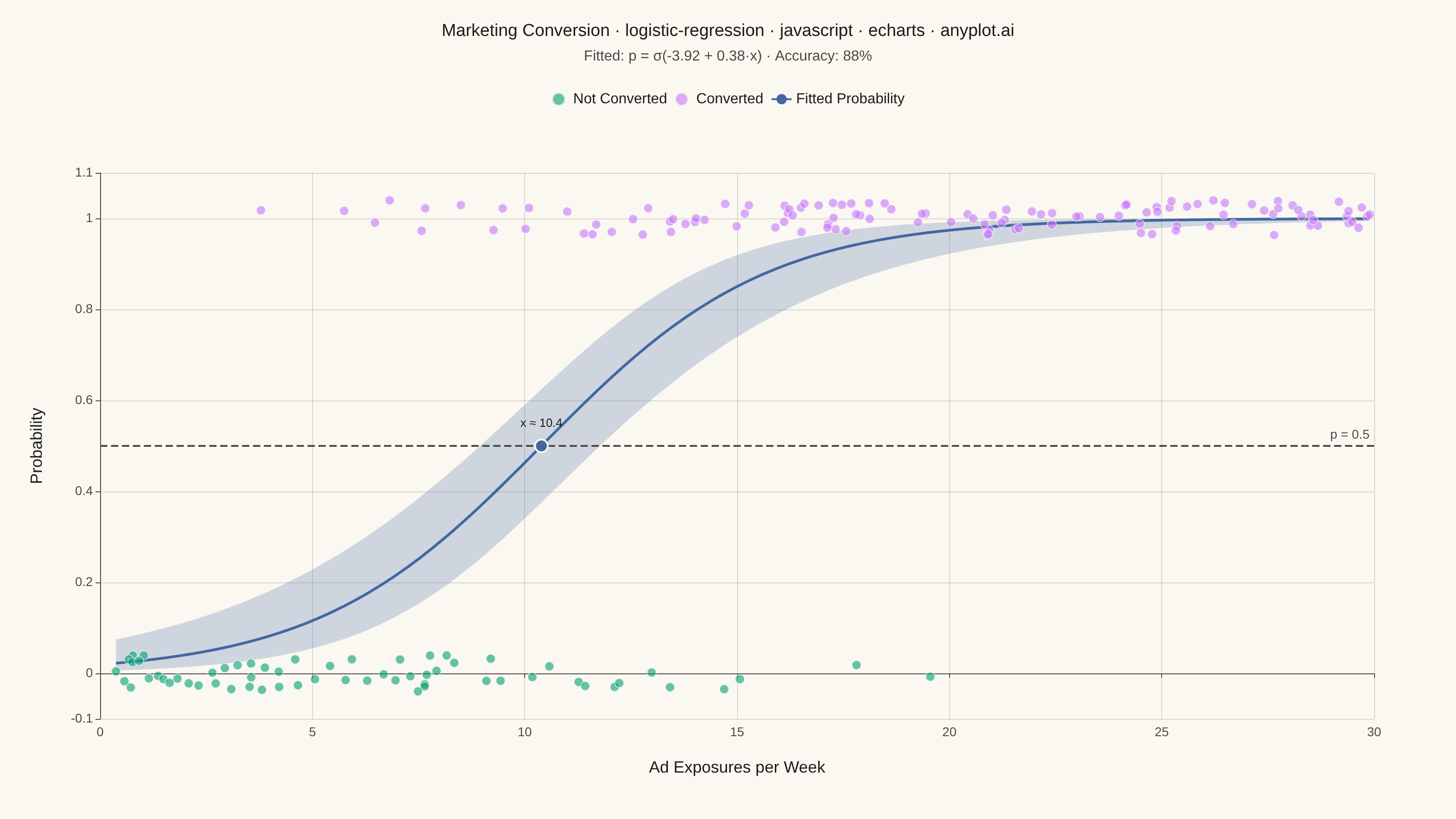
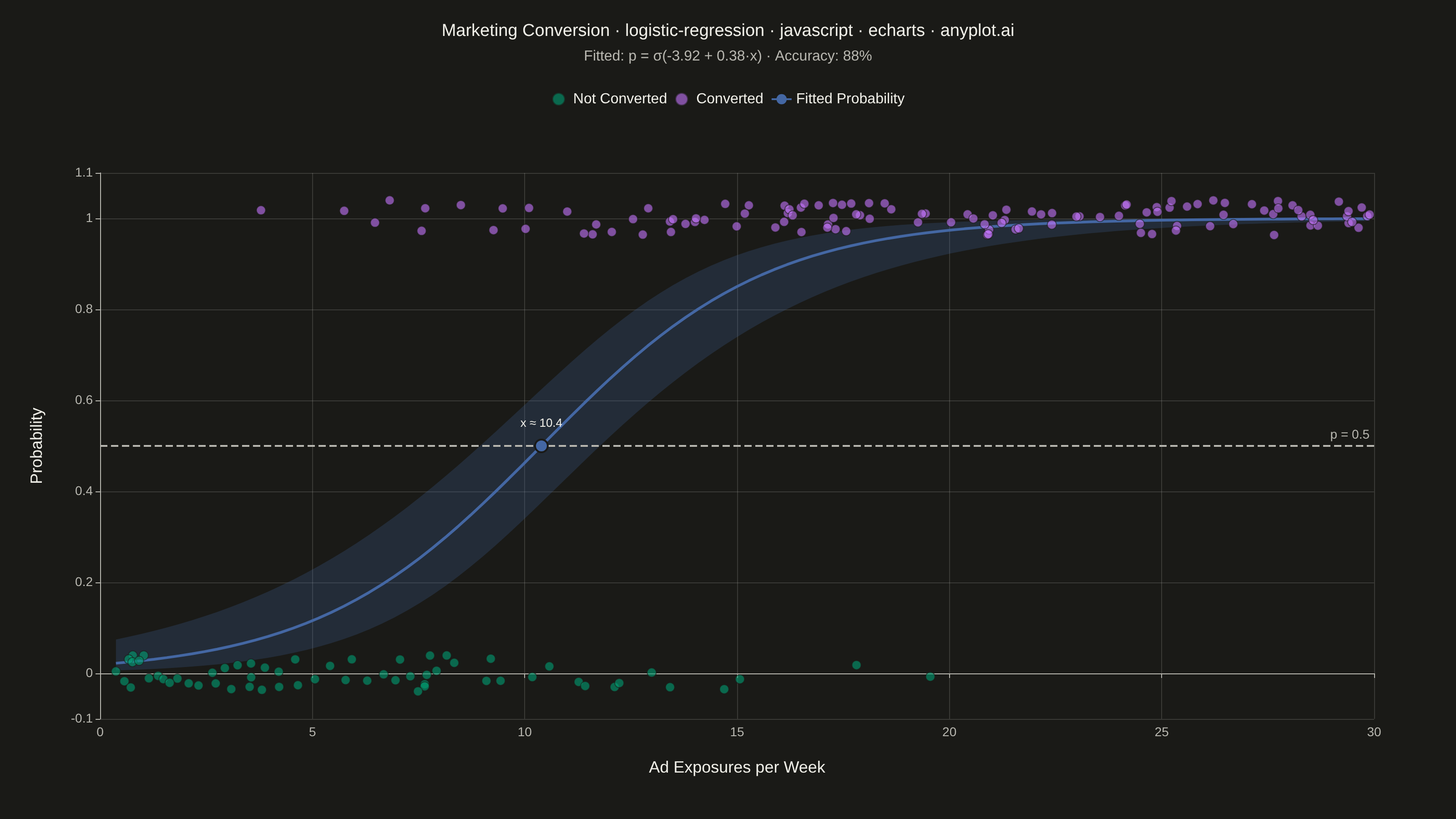
The same plot in 14 other libraries — JavaScript: Chart.js, D3.js, Highcharts, MUI X Charts; Python: Altair, Bokeh, lets-plot, Matplotlib, Plotly, plotnine, Pygal, Seaborn; R: ggplot2; Julia: Makie.jl. Compare all 15 side by side: Logistic Regression Curve Plot in Python, R, Julia and JavaScript.
A logistic regression visualization showing the characteristic S-shaped (sigmoid) probability curve for binary classification. The plot displays data points colored by their binary class, the fitted logistic curve representing predicted probabilities, confidence intervals around the curve, and a dashed decision threshold line at probability 0.5. This visualization is essential for understanding how a logistic model maps continuous input features to class probabilities.
// anyplot.ai
// logistic-regression: Logistic Regression Curve Plot
// Library: echarts 6.1.0 | JavaScript 22.23.2
// Quality: 89/100 | Created: 2026-09-02

const t = window.ANYPLOT_TOKENS;

// --- Data (in-memory, deterministic) ----------------------------------------
// A tiny fixed-seed LCG stands in for a seeded RNG (the browser has none).
function makeLcg(seed) {
  let state = seed >>> 0;
  return function () {
    state = (state * 1664525 + 1013904223) >>> 0;
    return state / 4294967296;
  };
}
const rand = makeLcg(42);

const N = 180;
const X_DOMAIN_MAX = 30;
const TRUE_BETA0 = -3.5;
const TRUE_BETA1 = 0.35; // ad exposures per week -> conversion probability

const sigmoid = (z) => 1 / (1 + Math.exp(-z));

const adExposures = Array.from({ length: N }, () => rand() * X_DOMAIN_MAX);
const converted = adExposures.map((x) => (rand() < sigmoid(TRUE_BETA0 + TRUE_BETA1 * x) ? 1 : 0));

// Jitter the binary outcome around 0/1 so overlapping points stay visible.
const notConvertedPoints = [];
const convertedPoints = [];
adExposures.forEach((x, i) => {
  const jitter = (rand() - 0.5) * 0.08;
  const point = [x, converted[i] + jitter];
  if (converted[i] === 1) convertedPoints.push(point);
  else notConvertedPoints.push(point);
});

// --- Fit a logistic regression via full-batch gradient descent -------------
const xMean = adExposures.reduce((a, b) => a + b, 0) / N;
const xStd = Math.sqrt(adExposures.reduce((a, x) => a + (x - xMean) ** 2, 0) / N);
const xNorm = adExposures.map((x) => (x - xMean) / xStd);

let w0 = 0;
let w1 = 0;
const LEARNING_RATE = 0.5;
for (let iter = 0; iter < 4000; iter++) {
  let grad0 = 0;
  let grad1 = 0;
  for (let i = 0; i < N; i++) {
    const p = sigmoid(w0 + w1 * xNorm[i]);
    const err = p - converted[i];
    grad0 += err;
    grad1 += err * xNorm[i];
  }
  w0 -= (LEARNING_RATE * grad0) / N;
  w1 -= (LEARNING_RATE * grad1) / N;
}

// Fisher information (Hessian of the log-likelihood) at the fitted weights,
// inverted analytically to get the asymptotic covariance of (w0, w1).
let h00 = 0;
let h01 = 0;
let h11 = 0;
for (let i = 0; i < N; i++) {
  const p = sigmoid(w0 + w1 * xNorm[i]);
  const wgt = p * (1 - p);
  h00 += wgt;
  h01 += wgt * xNorm[i];
  h11 += wgt * xNorm[i] * xNorm[i];
}
const det = h00 * h11 - h01 * h01;
const cov00 = h11 / det;
const cov01 = -h01 / det;
const cov11 = h00 / det;

// Real-scale coefficients (undo the x-normalization) for the annotation.
const realBeta1 = w1 / xStd;
const realBeta0 = w0 - (w1 * xMean) / xStd;
const accuracy =
  adExposures.reduce((correct, x, i) => {
    const predicted = sigmoid(realBeta0 + realBeta1 * x) > 0.5 ? 1 : 0;
    return correct + (predicted === converted[i] ? 1 : 0);
  }, 0) / N;

// --- Fitted curve + 95% confidence band (logit-scale, mapped back to prob) --
const CURVE_POINTS = 100;
const xMin = Math.min(...adExposures);
const xMax = Math.max(...adExposures);
const curveFit = [];
const curveLower = [];
const curveBandHeight = [];
for (let i = 0; i < CURVE_POINTS; i++) {
  const x = xMin + ((xMax - xMin) * i) / (CURVE_POINTS - 1);
  const xn = (x - xMean) / xStd;
  const eta = w0 + w1 * xn;
  const varEta = cov00 + 2 * xn * cov01 + xn * xn * cov11;
  const se = Math.sqrt(Math.max(varEta, 0));
  const pLo = sigmoid(eta - 1.96 * se);
  const pHi = sigmoid(eta + 1.96 * se);
  curveFit.push([x, sigmoid(eta)]);
  curveLower.push([x, pLo]);
  curveBandHeight.push([x, pHi - pLo]);
}

// x-value where the fitted curve crosses p = 0.5 (the decision threshold).
const xThreshold = -realBeta0 / realBeta1;

// --- Title (mandated format, fontsize scaled to the descriptive prefix) ----
const titleText = "Marketing Conversion · logistic-regression · javascript · echarts · anyplot.ai";
const titleRatio = titleText.length > 67 ? 67 / titleText.length : 1.0;
const titleFontSize = Math.max(14, Math.round(22 * titleRatio));
const subtext = `Fitted: p = σ(${realBeta0.toFixed(2)} + ${realBeta1.toFixed(2)}·x) · Accuracy: ${Math.round(accuracy * 100)}%`;

// --- Init ---------------------------------------------------------------
const chart = echarts.init(document.getElementById("container"));

// --- Option ---------------------------------------------------------------
chart.setOption({
  animation: false,
  backgroundColor: "transparent",
  color: t.palette,
  title: {
    text: titleText,
    subtext,
    left: "center",
    top: 20,
    textStyle: { color: t.ink, fontSize: titleFontSize, fontWeight: 500 },
    subtextStyle: { color: t.inkSoft, fontSize: 16 },
  },
  legend: {
    data: ["Not Converted", "Converted", "Fitted Probability"],
    top: 96,
    left: "center",
    textStyle: { color: t.ink, fontSize: 16 },
    itemWidth: 22,
    itemHeight: 14,
  },
  grid: { left: 110, right: 90, top: 190, bottom: 110 },
  xAxis: {
    type: "value",
    name: "Ad Exposures per Week",
    nameLocation: "middle",
    nameGap: 45,
    nameTextStyle: { color: t.ink, fontSize: 18 },
    min: 0,
    max: X_DOMAIN_MAX,
    axisLabel: { color: t.inkSoft, fontSize: 14 },
    axisLine: { lineStyle: { color: t.inkSoft } },
    splitLine: { lineStyle: { color: t.grid } },
  },
  yAxis: {
    type: "value",
    name: "Probability",
    nameLocation: "middle",
    nameGap: 60,
    nameTextStyle: { color: t.ink, fontSize: 18 },
    min: -0.1,
    max: 1.1,
    axisLabel: { color: t.inkSoft, fontSize: 14 },
    axisLine: { lineStyle: { color: t.inkSoft } },
    splitLine: { lineStyle: { color: t.grid } },
  },
  series: [
    {
      name: "ci-lower",
      type: "line",
      data: curveLower,
      stack: "confidence",
      symbol: "none",
      lineStyle: { opacity: 0 },
      areaStyle: { opacity: 0 },
      silent: true,
      tooltip: { show: false },
      z: 1,
    },
    {
      name: "ci-band",
      type: "line",
      data: curveBandHeight,
      stack: "confidence",
      symbol: "none",
      lineStyle: { opacity: 0 },
      areaStyle: { color: t.palette[2], opacity: 0.24 },
      silent: true,
      tooltip: { show: false },
      z: 1,
    },
    {
      name: "Not Converted",
      type: "scatter",
      data: notConvertedPoints,
      symbolSize: 10,
      itemStyle: { color: t.palette[0], opacity: 0.6, borderColor: t.pageBg, borderWidth: 1 },
      z: 3,
    },
    {
      name: "Converted",
      type: "scatter",
      data: convertedPoints,
      symbolSize: 10,
      itemStyle: { color: t.palette[1], opacity: 0.6, borderColor: t.pageBg, borderWidth: 1 },
      z: 3,
    },
    {
      name: "Fitted Probability",
      type: "line",
      data: curveFit,
      symbol: "none",
      lineStyle: { color: t.palette[2], width: 3 },
      z: 2,
      markLine: {
        silent: true,
        symbol: "none",
        lineStyle: { type: "dashed", color: t.inkSoft, width: 2 },
        label: { formatter: "p = 0.5", color: t.inkSoft, fontSize: 14, position: "insideEndTop" },
        data: [{ yAxis: 0.5 }],
      },
      markPoint: {
        silent: true,
        symbol: "circle",
        symbolSize: 14,
        itemStyle: { color: t.palette[2], borderColor: t.pageBg, borderWidth: 2 },
        label: {
          formatter: `x ≈ ${xThreshold.toFixed(1)}`,
          color: t.ink,
          fontSize: 13,
          position: "top",
          distance: 10,
        },
        data: [{ coord: [xThreshold, 0.5] }],
      },
    },
  ],
});
Runnable source as JSON, for any HTTP client: https://api.anyplot.ai/specs/logistic-regression/echarts/code. Any spec id and library id listed in llms-full.txt fit the same URL shape; every URL below is complete and callable.
{
  "spec_id": "logistic-regression",
  "language": "javascript",
  "library": "echarts",
  "page": "https://anyplot.ai/logistic-regression/javascript/echarts",
  "hub": "https://anyplot.ai/logistic-regression",
  "code_json": "https://api.anyplot.ai/specs/logistic-regression/echarts/code",
  "spec_json": "https://api.anyplot.ai/specs/logistic-regression",
  "render_light_png": "https://storage.googleapis.com/anyplot-images/plots/logistic-regression/javascript/echarts/plot-light.png",
  "render_dark_png": "https://storage.googleapis.com/anyplot-images/plots/logistic-regression/javascript/echarts/plot-dark.png",
  "interactive_light_html": "https://storage.googleapis.com/anyplot-images/plots/logistic-regression/javascript/echarts/plot-light.html",
  "interactive_dark_html": "https://storage.googleapis.com/anyplot-images/plots/logistic-regression/javascript/echarts/plot-dark.html",
  "quality_score": 89.0,
  "license": "MIT",
  "guide": "https://anyplot.ai/llms.txt"
}
Part of Logistic Regression Curve Plot on anyplot.ai.