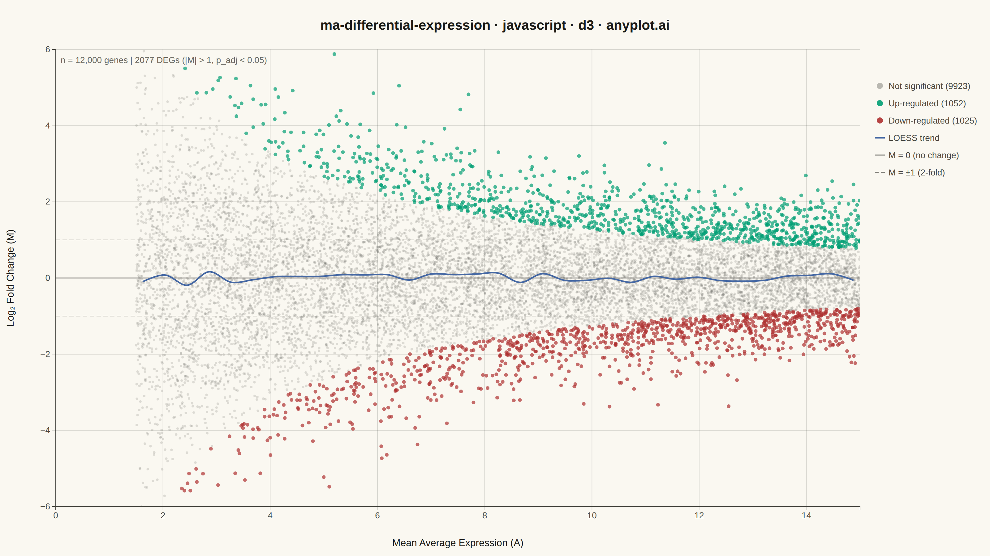
The same plot in 14 other libraries — JavaScript: Chart.js, Apache ECharts, Highcharts, MUI X Charts; Python: Altair, Bokeh, lets-plot, Matplotlib, Plotly, plotnine, Pygal, Seaborn; R: ggplot2; Julia: Makie.jl. Compare all 15 side by side: MA Plot for Differential Expression in Python, R, Julia and JavaScript.
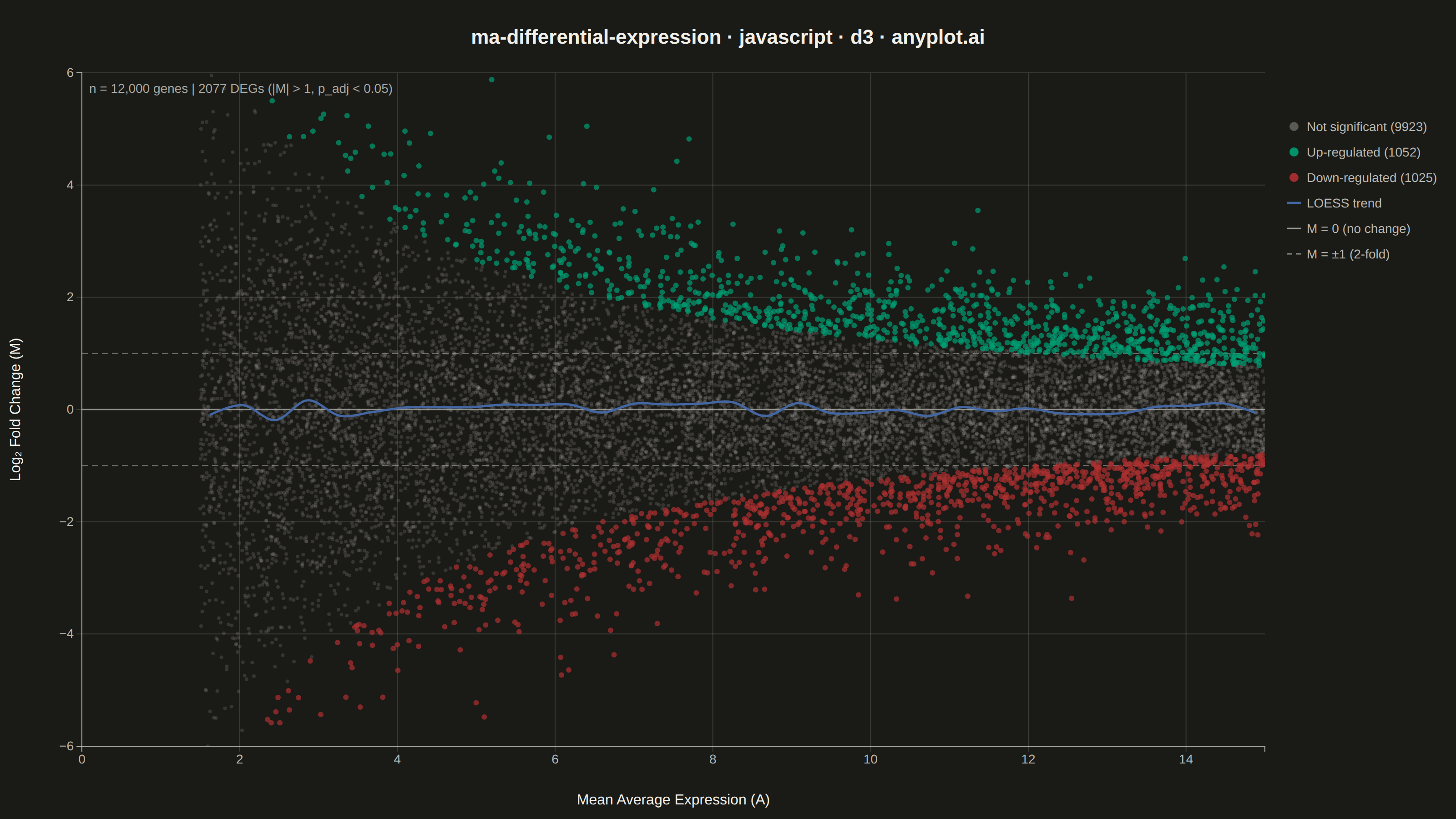
An MA plot (M-versus-A plot) visualizes the relationship between log fold change (M) and mean average expression (A) when comparing two experimental conditions. Each point represents a gene or feature, with significantly differentially expressed genes highlighted. This plot is a standard diagnostic tool in RNA-seq and microarray analysis for assessing differential expression results and detecting systematic expression-dependent bias.
// anyplot.ai
// ma-differential-expression: MA Plot for Differential Expression
// Library: d3 7.9.0 | JavaScript 22.22.3
// Quality: 88/100 | Created: 2026-06-21

const t = window.ANYPLOT_TOKENS;
const THEME = window.ANYPLOT_THEME;
const { width, height } = window.ANYPLOT_SIZE;

// Theme-adaptive muted color for non-significant genes
const INK_MUTED = THEME === "light" ? "#6B6A63" : "#A8A79F";

const margin = { top: 80, right: 210, bottom: 80, left: 90 };
const iw = width - margin.left - margin.right;
const ih = height - margin.top - margin.bottom;

// --- Deterministic LCG RNG ---
let seed = 42;
function rand() {
  seed = (seed * 1664525 + 1013904223) >>> 0;
  return seed / 4294967295;
}
function randn() {
  const u1 = Math.max(rand(), 1e-10);
  const u2 = rand();
  return Math.sqrt(-2 * Math.log(u1)) * Math.cos(2 * Math.PI * u2);
}

// --- Gene expression data (RNA-seq differential expression scenario) ---
// Treatment vs Control: 12000 genes, simulating DESeq2-style results
const N = 12000;
const genes = [];
for (let i = 0; i < N; i++) {
  const meanExpr = rand() * 13.5 + 1.5;        // baseMean: 1.5–15 (log2 CPM)
  const spread = 3.2 / (1 + meanExpr * 0.2);   // heteroscedasticity: low expr → high variance
  const lfc = randn() * spread;
  // Significance proxy: large fold-change with sufficient expression
  const zStat = Math.abs(lfc) / spread * Math.sqrt(meanExpr * 0.45);
  const significant = zStat > 2.5;
  genes.push({ meanExpr, lfc, significant, up: lfc > 0 });
}

// --- Binned smoothing (LOESS approximation via bin medians) ---
const nBins = 35;
const xBinMin = 1, xBinMax = 15.5;
const bw = (xBinMax - xBinMin) / nBins;
const bins = Array.from({ length: nBins }, (_, i) => ({
  x: xBinMin + (i + 0.5) * bw,
  ys: [],
}));
for (const gene of genes) {
  const bi = Math.min(nBins - 1, Math.floor((gene.meanExpr - xBinMin) / bw));
  if (bi >= 0) bins[bi].ys.push(gene.lfc);
}
const smoothCurve = bins
  .filter((b) => b.ys.length >= 5)
  .map((b) => {
    const sorted = [...b.ys].sort((a, c) => a - c);
    return { x: b.x, y: sorted[Math.floor(sorted.length / 2)] };
  });

// --- SVG mount ---
const svg = d3.select("#container").append("svg")
  .attr("width", width).attr("height", height);

// Clip path to contain scatter points within the plot area
svg.append("defs").append("clipPath").attr("id", "ma-clip")
  .append("rect").attr("width", iw).attr("height", ih);

const g = svg.append("g").attr("transform", `translate(${margin.left},${margin.top})`);

// --- Scales ---
const x = d3.scaleLinear().domain([0, 15]).range([0, iw]);
const y = d3.scaleLinear().domain([-6, 6]).range([ih, 0]);

// --- Grid lines (both axes for scatter plots per style guide) ---
g.append("g").selectAll(".grid-y")
  .data(y.ticks(8))
  .join("line")
  .attr("x1", 0).attr("x2", iw)
  .attr("y1", (d) => y(d)).attr("y2", (d) => y(d))
  .attr("stroke", t.grid).attr("stroke-width", 1);

g.append("g").selectAll(".grid-x")
  .data(x.ticks(8))
  .join("line")
  .attr("x1", (d) => x(d)).attr("x2", (d) => x(d))
  .attr("y1", 0).attr("y2", ih)
  .attr("stroke", t.grid).attr("stroke-width", 1);

// --- Reference lines ---
// M = 0: no change line
g.append("line")
  .attr("x1", 0).attr("x2", iw)
  .attr("y1", y(0)).attr("y2", y(0))
  .attr("stroke", t.ink).attr("stroke-width", 1.5).attr("opacity", 0.45);

// M = ±1: 2-fold change thresholds (dashed)
for (const m of [1, -1]) {
  g.append("line")
    .attr("x1", 0).attr("x2", iw)
    .attr("y1", y(m)).attr("y2", y(m))
    .attr("stroke", t.inkSoft).attr("stroke-width", 1)
    .attr("stroke-dasharray", "7 4").attr("opacity", 0.55);
}

// --- Scatter: draw in layers (non-sig background, then sig foreground) ---
const gClip = g.append("g").attr("clip-path", "url(#ma-clip)");

const nonsig = genes.filter((d) => !d.significant);
const upGenes = genes.filter((d) => d.significant && d.up);
const downGenes = genes.filter((d) => d.significant && !d.up);

// Non-significant genes (muted, semi-transparent background layer)
gClip.selectAll(".ns").data(nonsig).join("circle")
  .attr("cx", (d) => x(d.meanExpr)).attr("cy", (d) => y(d.lfc))
  .attr("r", 2).attr("fill", INK_MUTED).attr("opacity", 0.2);

// Down-regulated DEGs (matte red — semantic: loss/negative/down)
gClip.selectAll(".down").data(downGenes).join("circle")
  .attr("cx", (d) => x(d.meanExpr)).attr("cy", (d) => y(d.lfc))
  .attr("r", 3).attr("fill", t.palette[4]).attr("opacity", 0.7);

// Up-regulated DEGs (brand green — semantic: gain/positive/up)
gClip.selectAll(".up").data(upGenes).join("circle")
  .attr("cx", (d) => x(d.meanExpr)).attr("cy", (d) => y(d.lfc))
  .attr("r", 3).attr("fill", t.palette[0]).attr("opacity", 0.7);

// --- LOESS trend curve (bin median, smoothed with Catmull-Rom spline) ---
const smooth = d3.line()
  .x((d) => x(d.x)).y((d) => y(d.y))
  .curve(d3.curveCatmullRom);

gClip.append("path")
  .datum(smoothCurve)
  .attr("fill", "none")
  .attr("stroke", t.palette[2])
  .attr("stroke-width", 2.5)
  .attr("d", smooth);

// --- Axes ---
const xAx = g.append("g")
  .attr("transform", `translate(0,${ih})`)
  .call(d3.axisBottom(x).ticks(8));
const yAx = g.append("g")
  .call(d3.axisLeft(y).ticks(8));

for (const ax of [xAx, yAx]) {
  ax.selectAll("text").attr("fill", t.inkSoft).style("font-size", "14px");
  ax.selectAll("line").attr("stroke", t.grid);
  ax.select(".domain").attr("stroke", t.inkSoft);
}

// --- Axis labels ---
svg.append("text")
  .attr("x", margin.left + iw / 2).attr("y", height - 16)
  .attr("text-anchor", "middle").attr("fill", t.ink).style("font-size", "16px")
  .text("Mean Average Expression (A)");

svg.append("text")
  .attr("transform", "rotate(-90)")
  .attr("x", -(margin.top + ih / 2)).attr("y", 22)
  .attr("text-anchor", "middle").attr("fill", t.ink).style("font-size", "16px")
  .text("Log₂ Fold Change (M)");

// --- Legend ---
const legX = margin.left + iw + 24;
const legY = margin.top + 50;
const legG = svg.append("g").attr("transform", `translate(${legX},${legY})`);

const nSig = upGenes.length + downGenes.length;
const legItems = [
  { label: `Not significant (${nonsig.length})`, type: "dot", color: INK_MUTED, opacity: 0.45 },
  { label: `Up-regulated (${upGenes.length})`, type: "dot", color: t.palette[0], opacity: 0.9 },
  { label: `Down-regulated (${downGenes.length})`, type: "dot", color: t.palette[4], opacity: 0.9 },
  { label: "LOESS trend", type: "line", color: t.palette[2], opacity: 1 },
  { label: "M = 0 (no change)", type: "solid", color: t.ink, opacity: 0.6 },
  { label: "M = ±1 (2-fold)", type: "dashed", color: t.inkSoft, opacity: 0.7 },
];

legItems.forEach((item, i) => {
  const row = legG.append("g").attr("transform", `translate(0,${i * 28})`);
  if (item.type === "dot") {
    row.append("circle")
      .attr("cx", 8).attr("cy", 9).attr("r", 5)
      .attr("fill", item.color).attr("opacity", item.opacity);
  } else {
    row.append("line")
      .attr("x1", 0).attr("x2", 16).attr("y1", 9).attr("y2", 9)
      .attr("stroke", item.color)
      .attr("stroke-width", item.type === "line" ? 2.5 : 1.5)
      .attr("stroke-dasharray", item.type === "dashed" ? "6 4" : null)
      .attr("opacity", item.opacity);
  }
  row.append("text")
    .attr("x", 22).attr("y", 14)
    .attr("fill", t.inkSoft).style("font-size", "14px")
    .text(item.label);
});

// --- Gene count annotation ---
svg.append("text")
  .attr("x", margin.left + 8).attr("y", margin.top + 22)
  .attr("fill", INK_MUTED).style("font-size", "14px")
  .text(`n = ${N.toLocaleString()} genes | ${nSig} DEGs (|M| > 1, p_adj < 0.05)`);

// --- Title ---
const title = "ma-differential-expression · javascript · d3 · anyplot.ai";
svg.append("text")
  .attr("x", width / 2).attr("y", 48)
  .attr("text-anchor", "middle").attr("fill", t.ink)
  .style("font-size", "22px").style("font-weight", "600")
  .text(title);
Runnable source as JSON, for any HTTP client: https://api.anyplot.ai/specs/ma-differential-expression/d3/code. Any spec id and library id listed in llms-full.txt fit the same URL shape; every URL below is complete and callable.
{
  "spec_id": "ma-differential-expression",
  "language": "javascript",
  "library": "d3",
  "page": "https://anyplot.ai/ma-differential-expression/javascript/d3",
  "hub": "https://anyplot.ai/ma-differential-expression",
  "code_json": "https://api.anyplot.ai/specs/ma-differential-expression/d3/code",
  "spec_json": "https://api.anyplot.ai/specs/ma-differential-expression",
  "render_light_png": "https://storage.googleapis.com/anyplot-images/plots/ma-differential-expression/javascript/d3/plot-light.png",
  "render_dark_png": "https://storage.googleapis.com/anyplot-images/plots/ma-differential-expression/javascript/d3/plot-dark.png",
  "interactive_light_html": "https://storage.googleapis.com/anyplot-images/plots/ma-differential-expression/javascript/d3/plot-light.html",
  "interactive_dark_html": "https://storage.googleapis.com/anyplot-images/plots/ma-differential-expression/javascript/d3/plot-dark.html",
  "quality_score": 88.0,
  "license": "MIT",
  "guide": "https://anyplot.ai/llms.txt"
}
Part of MA Plot for Differential Expression on anyplot.ai.