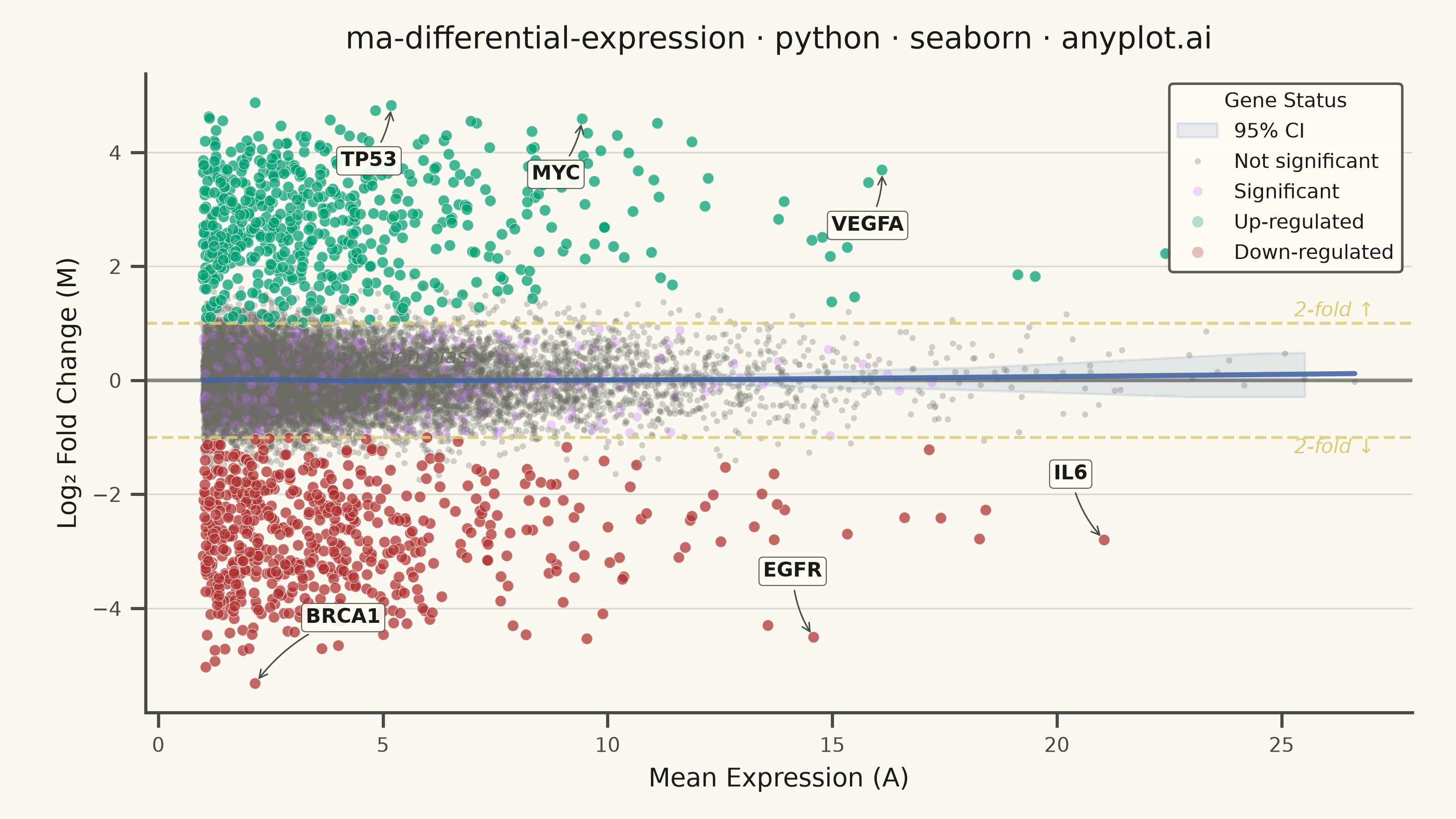
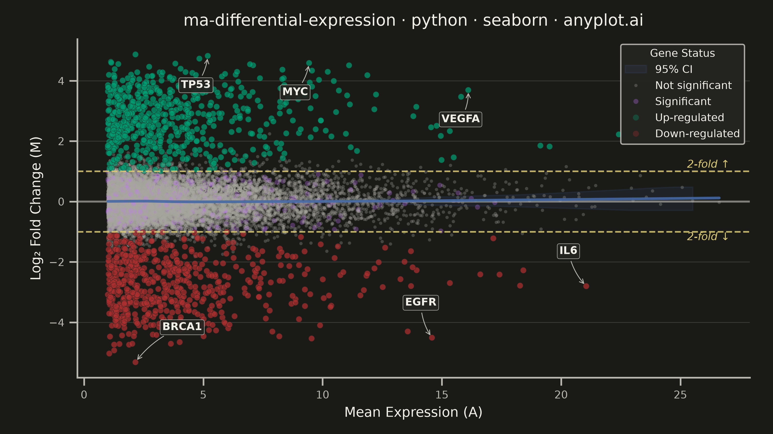
An MA plot (M-versus-A plot) visualizes the relationship between log fold change (M) and mean average expression (A) when comparing two experimental conditions. Each point represents a gene or feature, with significantly differentially expressed genes highlighted. This plot is a standard diagnostic tool in RNA-seq and microarray analysis for assessing differential expression results and detecting systematic expression-dependent bias.
""" anyplot.ai
ma-differential-expression: MA Plot for Differential Expression
Library: seaborn 0.13.2 | Python 3.13.14
Quality: 88/100 | Updated: 2026-06-21
"""

import os
import sys


# Remove the script's own directory from sys.path so that sibling files
# (matplotlib.py, seaborn.py, etc.) don't shadow installed packages.
try:
    _here = os.path.realpath(os.path.dirname(__file__))
except NameError:
    _here = os.path.realpath(os.getcwd())
sys.path = [p for p in sys.path if p and os.path.realpath(p) != _here]

import matplotlib.pyplot as plt
import numpy as np
import pandas as pd
import seaborn as sns
from statsmodels.nonparametric.smoothers_lowess import lowess as sm_lowess


THEME = os.getenv("ANYPLOT_THEME", "light")

PAGE_BG = "#FAF8F1" if THEME == "light" else "#1A1A17"
ELEVATED_BG = "#FFFDF6" if THEME == "light" else "#242420"
INK = "#1A1A17" if THEME == "light" else "#F0EFE8"
INK_SOFT = "#4A4A44" if THEME == "light" else "#B8B7B0"
INK_MUTED = "#6B6A63" if THEME == "light" else "#A8A79F"

# Imprint palette — canonical order, first series always #009E73
IMPRINT_PALETTE = ["#009E73", "#C475FD", "#4467A3", "#BD8233", "#AE3030", "#2ABCCD", "#954477", "#99B314"]
ANYPLOT_AMBER = "#DDCC77"  # warning / caution (outside categorical pool)

# Semantic mapping: up=green (positive/gain), down=matte-red (loss/negative)
UP_COLOR = IMPRINT_PALETTE[0]  # #009E73 — first Imprint series, semantically "positive/up"
SIG_COLOR = IMPRINT_PALETTE[1]  # #C475FD lavender — significant but sub-threshold fold change
DOWN_COLOR = IMPRINT_PALETTE[4]  # #AE3030 matte red — semantic anchor for loss/negative
NSIG_COLOR = INK_MUTED  # theme-adaptive muted gray for background noise

LOESS_COLOR = IMPRINT_PALETTE[2]  # #4467A3 blue — trend overlay
THRESHOLD_COLOR = ANYPLOT_AMBER  # #DDCC77 — caution/threshold lines

sns.set_theme(
    style="ticks",
    rc={
        "figure.facecolor": PAGE_BG,
        "axes.facecolor": PAGE_BG,
        "axes.edgecolor": INK_SOFT,
        "axes.labelcolor": INK,
        "text.color": INK,
        "xtick.color": INK_SOFT,
        "ytick.color": INK_SOFT,
        "grid.color": INK,
        "grid.alpha": 0.15,
        "legend.facecolor": ELEVATED_BG,
        "legend.edgecolor": INK_SOFT,
    },
)

# --- Data ---
np.random.seed(42)
n_genes = 15000

mean_expression = np.random.exponential(scale=3, size=n_genes) + 1
log_fold_change = np.random.normal(0, 0.5, n_genes)

n_de = int(n_genes * 0.08)
de_indices = np.random.choice(n_genes, n_de, replace=False)
log_fold_change[de_indices] += np.random.choice([-1, 1], n_de) * np.random.uniform(1.5, 4, n_de)

p_values = np.ones(n_genes)
p_values[de_indices] = 10 ** (-np.random.uniform(2, 10, n_de))
p_values[~np.isin(np.arange(n_genes), de_indices)] = np.random.uniform(0.01, 1.0, n_genes - n_de)

significant = p_values < 0.05

status = np.where(
    ~significant,
    "Not significant",
    np.where(log_fold_change > 1, "Up-regulated", np.where(log_fold_change < -1, "Down-regulated", "Significant")),
)

# Gene names spread across expression range for spatial storytelling
gene_names = [None] * n_genes
top_gene_labels = ["BRCA1", "TP53", "MYC", "EGFR", "VEGFA", "IL6"]
sig_de_mask = significant & (np.abs(log_fold_change) > 1)
sig_de_indices = np.where(sig_de_mask)[0]
sig_de_expr = mean_expression[sig_de_indices]
sig_de_abs_lfc = np.abs(log_fold_change[sig_de_indices])

expr_min, expr_max = sig_de_expr.min(), sig_de_expr.max()
n_labels = len(top_gene_labels)
expr_edges = np.linspace(expr_min, expr_max + 0.01, n_labels + 1)
top_sig = []
for b in range(n_labels):
    in_bin = (sig_de_expr >= expr_edges[b]) & (sig_de_expr < expr_edges[b + 1])
    if not np.any(in_bin):
        continue
    bin_idx = np.where(in_bin)[0]
    best = bin_idx[np.argmax(sig_de_abs_lfc[bin_idx])]
    top_sig.append(sig_de_indices[best])

for i, idx in enumerate(top_sig[:n_labels]):
    gene_names[idx] = top_gene_labels[i]

df = pd.DataFrame(
    {
        "Mean Expression (A)": mean_expression,
        "Log₂ Fold Change (M)": log_fold_change,
        "Status": pd.Categorical(
            status, categories=["Not significant", "Significant", "Up-regulated", "Down-regulated"]
        ),
        "gene_name": gene_names,
    }
)

status_palette = {
    "Not significant": NSIG_COLOR,
    "Significant": SIG_COLOR,
    "Up-regulated": UP_COLOR,
    "Down-regulated": DOWN_COLOR,
}

# --- Precompute LOESS + bootstrap CI (seaborn confidence-band pattern) ---
x_all = df["Mean Expression (A)"].values
y_all = df["Log₂ Fold Change (M)"].values
sort_full = np.argsort(x_all)
x_sorted, y_sorted = x_all[sort_full], y_all[sort_full]

# Full-data LOESS for annotation placement
loess_full = sm_lowess(y_sorted, x_sorted, frac=0.3, return_sorted=True)

# Bootstrap CI on 2k subsample for speed (pattern mirrors seaborn's CI bands)
rng_boot = np.random.default_rng(0)
sub_idx = np.sort(rng_boot.choice(len(x_sorted), 2000, replace=False))
xs_b, ys_b = x_sorted[sub_idx], y_sorted[sub_idx]
x_grid = np.linspace(xs_b[0], xs_b[-1], 200)

n_boot = 80
boot_curves = np.empty((n_boot, len(x_grid)))
for bi in range(n_boot):
    ri = rng_boot.integers(0, len(xs_b), len(xs_b))
    xr, yr = xs_b[ri], ys_b[ri]
    s = np.argsort(xr)
    lw = sm_lowess(yr[s], xr[s], frac=0.3, return_sorted=True)
    boot_curves[bi] = np.interp(x_grid, lw[:, 0], lw[:, 1])

ci_lo = np.percentile(boot_curves, 2.5, axis=0)
ci_hi = np.percentile(boot_curves, 97.5, axis=0)

# --- Plot ---
fig, ax = plt.subplots(figsize=(8, 4.5), dpi=400)
fig.patch.set_facecolor(PAGE_BG)
ax.set_facecolor(PAGE_BG)

# LOESS 95% CI band drawn first so data points render on top
ax.fill_between(x_grid, ci_lo, ci_hi, color=LOESS_COLOR, alpha=0.12, zorder=1, label="95% CI")

# Reference lines
ax.axhline(y=0, color=INK_SOFT, linewidth=1.5, alpha=0.6, zorder=2)
ax.axhline(y=1, color=THRESHOLD_COLOR, linewidth=1.2, linestyle="--", alpha=0.85, zorder=2)
ax.axhline(y=-1, color=THRESHOLD_COLOR, linewidth=1.2, linestyle="--", alpha=0.85, zorder=2)

# Background layer: all 15k genes, small + transparent for density
sns.scatterplot(
    data=df,
    x="Mean Expression (A)",
    y="Log₂ Fold Change (M)",
    hue="Status",
    hue_order=["Not significant", "Significant", "Up-regulated", "Down-regulated"],
    palette=status_palette,
    size="Status",
    sizes={"Not significant": 6, "Significant": 14, "Up-regulated": 20, "Down-regulated": 20},
    alpha=0.3,
    edgecolor="none",
    legend="full",
    ax=ax,
)

# Emphasis layer: DE genes with subtle edge for definition
de_data = df[df["Status"].isin(["Up-regulated", "Down-regulated"])]
sns.scatterplot(
    data=de_data,
    x="Mean Expression (A)",
    y="Log₂ Fold Change (M)",
    hue="Status",
    hue_order=["Up-regulated", "Down-regulated"],
    palette={"Up-regulated": UP_COLOR, "Down-regulated": DOWN_COLOR},
    s=20,
    alpha=0.6,
    edgecolor=ELEVATED_BG,
    linewidth=0.3,
    legend=False,
    ax=ax,
)

# Threshold annotations (raised to 8pt for mobile legibility)
xlim = ax.get_xlim()
x_lbl = xlim[1] * 0.97
ax.text(x_lbl, 1.12, "2-fold ↑", fontsize=8, color=THRESHOLD_COLOR, ha="right", fontstyle="italic")
ax.text(x_lbl, -1.28, "2-fold ↓", fontsize=8, color=THRESHOLD_COLOR, ha="right", fontstyle="italic")

# LOESS smoothing curve (seaborn-distinctive lowess via regplot)
sns.regplot(
    data=df,
    x="Mean Expression (A)",
    y="Log₂ Fold Change (M)",
    lowess=True,
    scatter=False,
    line_kws={"color": LOESS_COLOR, "linewidth": 2.0, "alpha": 0.9, "label": "LOESS trend"},
    ax=ax,
)

# In-plot annotation foregrounding the key finding: flat LOESS = no expression bias
x_annot = float(np.percentile(x_all, 86))
y_annot = float(np.interp(x_annot, loess_full[:, 0], loess_full[:, 1]))
ax.text(
    x_annot,
    y_annot + 0.22,
    "No expression bias",
    fontsize=8,
    fontstyle="italic",
    color=INK_MUTED,
    ha="right",
    va="bottom",
)

# Gene labels spread across expression range with refined offsets and thinner arrowheads
labeled = df[df["gene_name"].notna()].copy()
label_positions = []
for _, row in labeled.iterrows():
    x_val = row["Mean Expression (A)"]
    y_val = row["Log₂ Fold Change (M)"]
    y_off = -24 if y_val > 0 else 24
    x_off = 20 if x_val < df["Mean Expression (A)"].median() else -20
    for px, py in label_positions:
        if abs(x_val - px) < 2 and abs(y_val - py) < 1:
            y_off = y_off + (30 if y_off > 0 else -30)
            break
    label_positions.append((x_val, y_val))
    ax.annotate(
        row["gene_name"],
        xy=(x_val, y_val),
        xytext=(x_off, y_off),
        textcoords="offset points",
        fontsize=8,
        fontweight="bold",
        color=INK,
        arrowprops={"arrowstyle": "->", "color": INK_SOFT, "lw": 0.6, "connectionstyle": "arc3,rad=0.15"},
        bbox={
            "boxstyle": "round,pad=0.2",
            "facecolor": ELEVATED_BG,
            "edgecolor": INK_SOFT,
            "alpha": 0.92,
            "linewidth": 0.4,
        },
    )

# Style
sns.despine(ax=ax)
ax.set_xlabel("Mean Expression (A)", fontsize=10, color=INK)
ax.set_ylabel("Log₂ Fold Change (M)", fontsize=10, color=INK)
ax.set_title(
    "ma-differential-expression · python · seaborn · anyplot.ai", fontsize=12, fontweight="medium", pad=10, color=INK
)
ax.tick_params(axis="both", labelsize=8, colors=INK_SOFT)
ax.yaxis.grid(True, alpha=0.15, linewidth=0.6, color=INK)

sns.move_legend(ax, "upper right", fontsize=8, framealpha=0.92, title="Gene Status", title_fontsize=8)

fig.subplots_adjust(left=0.10, right=0.97, top=0.91, bottom=0.13)
plt.savefig(f"plot-{THEME}.png", dpi=400, facecolor=PAGE_BG)
plt.close()
Runnable source as JSON, for any HTTP client: https://api.anyplot.ai/specs/ma-differential-expression/seaborn/code. Any spec id and library id listed in llms-full.txt fit the same URL shape; every URL below is complete and callable.
{
  "spec_id": "ma-differential-expression",
  "language": "python",
  "library": "seaborn",
  "page": "https://anyplot.ai/ma-differential-expression/python/seaborn",
  "hub": "https://anyplot.ai/ma-differential-expression",
  "code_json": "https://api.anyplot.ai/specs/ma-differential-expression/seaborn/code",
  "spec_json": "https://api.anyplot.ai/specs/ma-differential-expression",
  "render_light_png": "https://storage.googleapis.com/anyplot-images/plots/ma-differential-expression/python/seaborn/plot-light.png",
  "render_dark_png": "https://storage.googleapis.com/anyplot-images/plots/ma-differential-expression/python/seaborn/plot-dark.png",
  "quality_score": 88.0,
  "license": "MIT",
  "guide": "https://anyplot.ai/llms.txt"
}
Part of MA Plot for Differential Expression on anyplot.ai.