The same plot in 14 other libraries — Python: Altair, Bokeh, lets-plot, Matplotlib, Plotly, plotnine, Pygal, Seaborn; R: ggplot2; JavaScript: Chart.js, D3.js, Apache ECharts, Highcharts, MUI X Charts. Compare all 15 side by side: MA Plot for Differential Expression in Python, R, Julia and JavaScript.
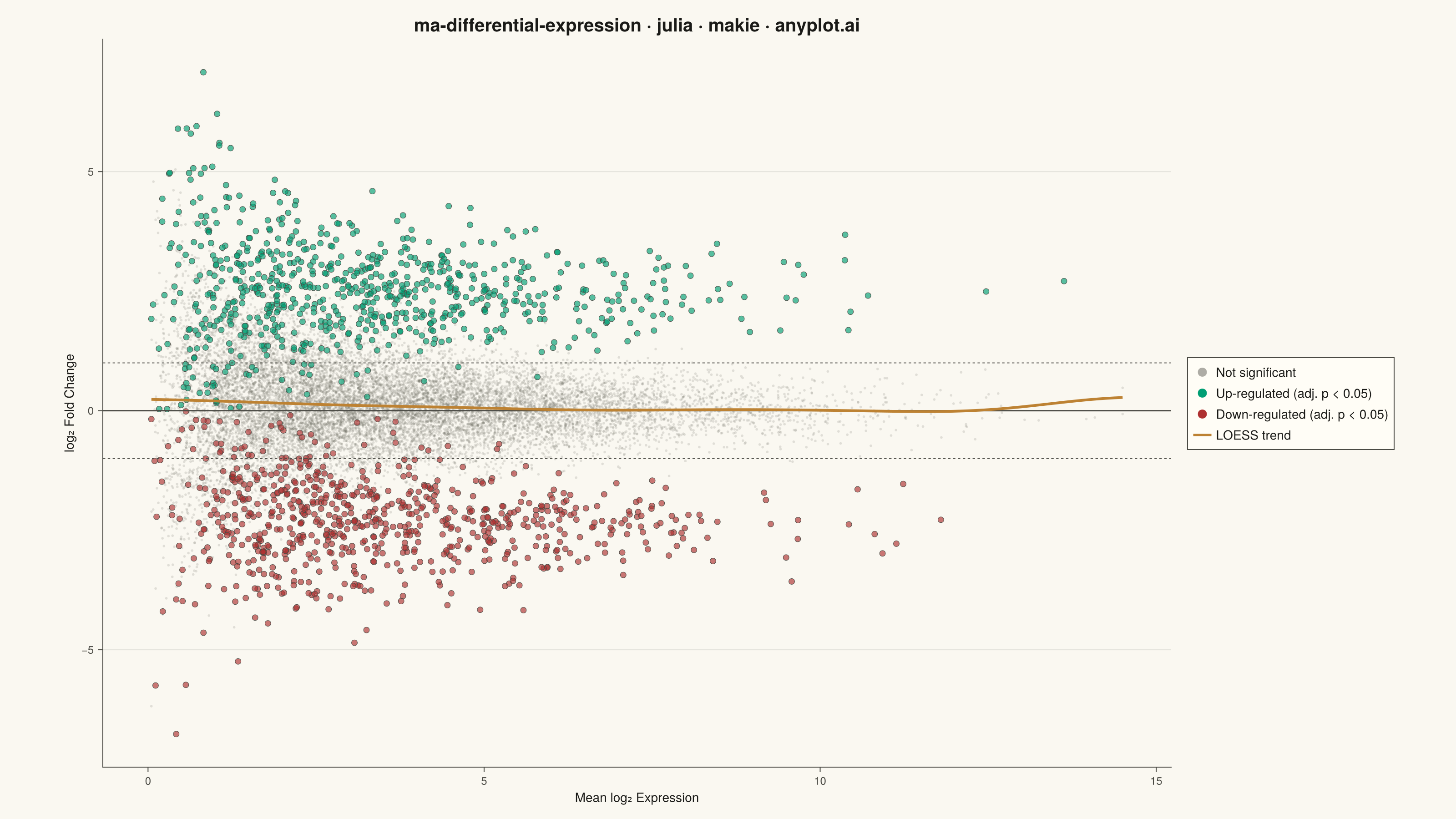
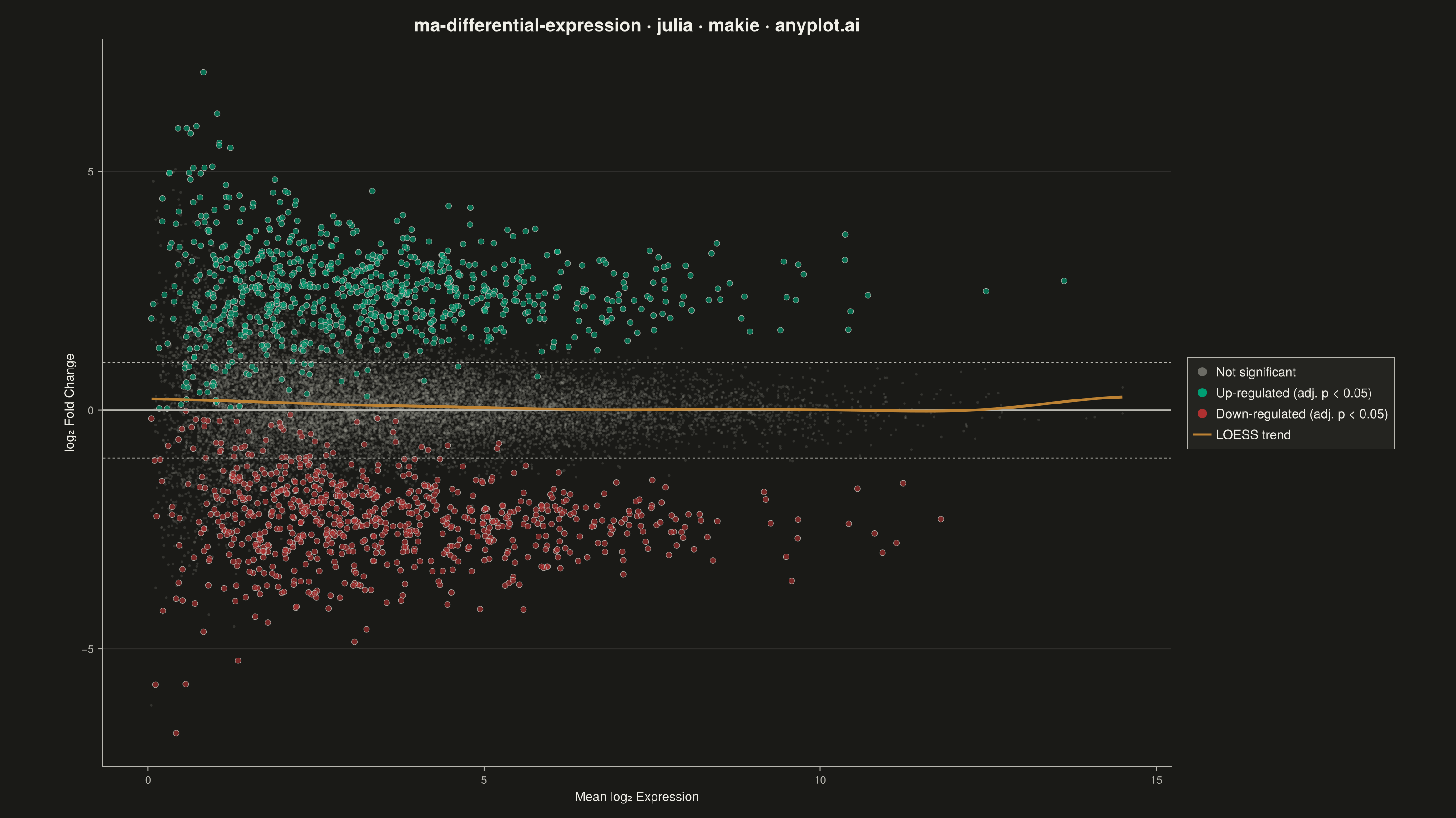
An MA plot (M-versus-A plot) visualizes the relationship between log fold change (M) and mean average expression (A) when comparing two experimental conditions. Each point represents a gene or feature, with significantly differentially expressed genes highlighted. This plot is a standard diagnostic tool in RNA-seq and microarray analysis for assessing differential expression results and detecting systematic expression-dependent bias.
# anyplot.ai
# ma-differential-expression: MA Plot for Differential Expression
# Library: makie 0.22.10 | Julia 1.11.9
# Quality: 88/100 | Created: 2026-06-21

using CairoMakie
using Colors
using Random

Random.seed!(42)

# Theme tokens
const THEME       = get(ENV, "ANYPLOT_THEME", "light")
const PAGE_BG     = THEME == "light" ? colorant"#FAF8F1" : colorant"#1A1A17"
const ELEVATED_BG = THEME == "light" ? colorant"#FFFDF6" : colorant"#242420"
const INK         = THEME == "light" ? colorant"#1A1A17" : colorant"#F0EFE8"
const INK_SOFT    = THEME == "light" ? colorant"#4A4A44" : colorant"#B8B7B0"
const INK_MUTED   = THEME == "light" ? colorant"#6B6A63" : colorant"#A8A79F"

# Imprint palette positions used in this plot
const BRAND_GREEN = colorant"#009E73"  # position 1 — up-regulated (gain)
const MATTE_RED   = colorant"#AE3030"  # semantic anchor — down-regulated (loss)
const OCHRE       = colorant"#BD8233"  # position 4 — LOESS trend line

# Data — simulated RNA-seq differential expression (~15 000 genes)
n_genes = 15_000

# A-values: mean log2 expression (funnel-shaped distribution typical of RNA-seq)
mean_expr = abs.(randn(n_genes)) .* 3.5 .+ abs.(randn(n_genes)) .* 1.0
mean_expr = clamp.(mean_expr, 0.05, 14.5)

# M-values: LFC variance shrinks at higher expression
lfc_noise = (2.0 ./ (mean_expr .+ 0.8)) .+ 0.18
lfc = randn(n_genes) .* lfc_noise

# Slight upward bias at low expression — common normalization artifact
lfc .+= 0.25 .* exp.(-mean_expr ./ 3.5)

# Inject ~10 % truly differentially expressed genes
n_de    = 1_500
de_idx  = randperm(n_genes)[1:n_de]
half_de = div(n_de, 2)
for i in 1:half_de
    lfc[de_idx[i]] += 1.9 + abs(randn()) * 0.6
end
for i in (half_de + 1):n_de
    lfc[de_idx[i]] -= 1.9 + abs(randn()) * 0.6
end
lfc = clamp.(lfc, -7.5, 7.5)

significant = falses(n_genes)
significant[de_idx] .= true

not_sig  = .!significant
sig_up   = significant .& (lfc .>  0.0)
sig_down = significant .& (lfc .<= 0.0)

# Gaussian kernel smoothing — LOESS approximation (inline, no function)
n_eval   = 120
bw       = 1.5
x_eval   = collect(range(minimum(mean_expr), maximum(mean_expr), length=n_eval))
y_smooth = zeros(n_eval)
for i in eachindex(x_eval)
    w       = exp.(-((mean_expr .- x_eval[i]) ./ bw) .^ 2)
    wsum    = sum(w)
    y_smooth[i] = wsum > 1e-10 ? sum(w .* lfc) / wsum : 0.0
end

# Figure
fig = Figure(
    size            = (1600, 900),
    fontsize        = 14,
    backgroundcolor = PAGE_BG,
)

ax = Axis(
    fig[1, 1];
    title              = "ma-differential-expression · julia · makie · anyplot.ai",
    titlesize          = 20,
    titlecolor         = INK,
    xlabel             = "Mean log₂ Expression",
    ylabel             = "log₂ Fold Change",
    xlabelsize         = 14,
    ylabelsize         = 14,
    xlabelcolor        = INK,
    ylabelcolor        = INK,
    xticklabelsize     = 12,
    yticklabelsize     = 12,
    xticklabelcolor    = INK_SOFT,
    yticklabelcolor    = INK_SOFT,
    xtickcolor         = INK_SOFT,
    ytickcolor         = INK_SOFT,
    backgroundcolor    = PAGE_BG,
    topspinevisible    = false,
    rightspinevisible  = false,
    leftspinecolor     = INK_SOFT,
    bottomspinecolor   = INK_SOFT,
    xgridvisible       = false,
    ygridcolor         = RGBAf(INK.r, INK.g, INK.b, 0.10),
    xminorgridvisible  = false,
    yminorgridvisible  = false,
)

# Layer 1: non-significant genes (large cloud, semi-transparent)
scatter!(ax, mean_expr[not_sig], lfc[not_sig];
    color       = (INK_MUTED, 0.18),
    markersize  = 4,
    strokewidth = 0,
)

# Layer 2: significantly up-regulated genes (brand green — gain)
scatter!(ax, mean_expr[sig_up], lfc[sig_up];
    color       = (BRAND_GREEN, 0.65),
    markersize  = 9,
    strokewidth = 0.5,
    strokecolor = INK_SOFT,
)

# Layer 3: significantly down-regulated genes (matte red — loss)
scatter!(ax, mean_expr[sig_down], lfc[sig_down];
    color       = (MATTE_RED, 0.65),
    markersize  = 9,
    strokewidth = 0.5,
    strokecolor = INK_SOFT,
)

# Reference lines: zero line and ±1 log2 FC thresholds
hlines!(ax, [0.0]; color = INK_SOFT, linewidth = 1.5)
hlines!(ax, [1.0, -1.0]; color = INK_SOFT, linewidth = 0.9, linestyle = :dash)

# LOESS-like smoothing curve
lines!(ax, x_eval, y_smooth; color = OCHRE, linewidth = 3.0)

# Legend
Legend(
    fig[1, 2],
    [
        MarkerElement(
            color = RGBAf(INK_MUTED.r, INK_MUTED.g, INK_MUTED.b, 0.55),
            marker = :circle, markersize = 14,
        ),
        MarkerElement(color = BRAND_GREEN, marker = :circle, markersize = 14),
        MarkerElement(color = MATTE_RED,   marker = :circle, markersize = 14),
        LineElement(color = OCHRE, linewidth = 2.5),
    ],
    [
        "Not significant",
        "Up-regulated (adj. p < 0.05)",
        "Down-regulated (adj. p < 0.05)",
        "LOESS trend",
    ],
    framevisible    = true,
    framecolor      = INK_SOFT,
    backgroundcolor = ELEVATED_BG,
    labelcolor      = INK,
    labelsize       = 14,
)

colsize!(fig.layout, 1, Relative(0.78))

# Save
save("plot-$(THEME).png", fig; px_per_unit = 2)
Runnable source as JSON, for any HTTP client: https://api.anyplot.ai/specs/ma-differential-expression/makie/code. Any spec id and library id listed in llms-full.txt fit the same URL shape; every URL below is complete and callable.
{
  "spec_id": "ma-differential-expression",
  "language": "julia",
  "library": "makie",
  "page": "https://anyplot.ai/ma-differential-expression/julia/makie",
  "hub": "https://anyplot.ai/ma-differential-expression",
  "code_json": "https://api.anyplot.ai/specs/ma-differential-expression/makie/code",
  "spec_json": "https://api.anyplot.ai/specs/ma-differential-expression",
  "render_light_png": "https://storage.googleapis.com/anyplot-images/plots/ma-differential-expression/julia/makie/plot-light.png",
  "render_dark_png": "https://storage.googleapis.com/anyplot-images/plots/ma-differential-expression/julia/makie/plot-dark.png",
  "quality_score": 88.0,
  "license": "MIT",
  "guide": "https://anyplot.ai/llms.txt"
}
Part of MA Plot for Differential Expression on anyplot.ai.