The same plot in 14 other libraries — Python: Altair, Bokeh, lets-plot, Matplotlib, Plotly, plotnine, Pygal, Seaborn; Julia: Makie.jl; JavaScript: Chart.js, D3.js, Apache ECharts, Highcharts, MUI X Charts. Compare all 15 side by side: MA Plot for Differential Expression in Python, R, Julia and JavaScript.
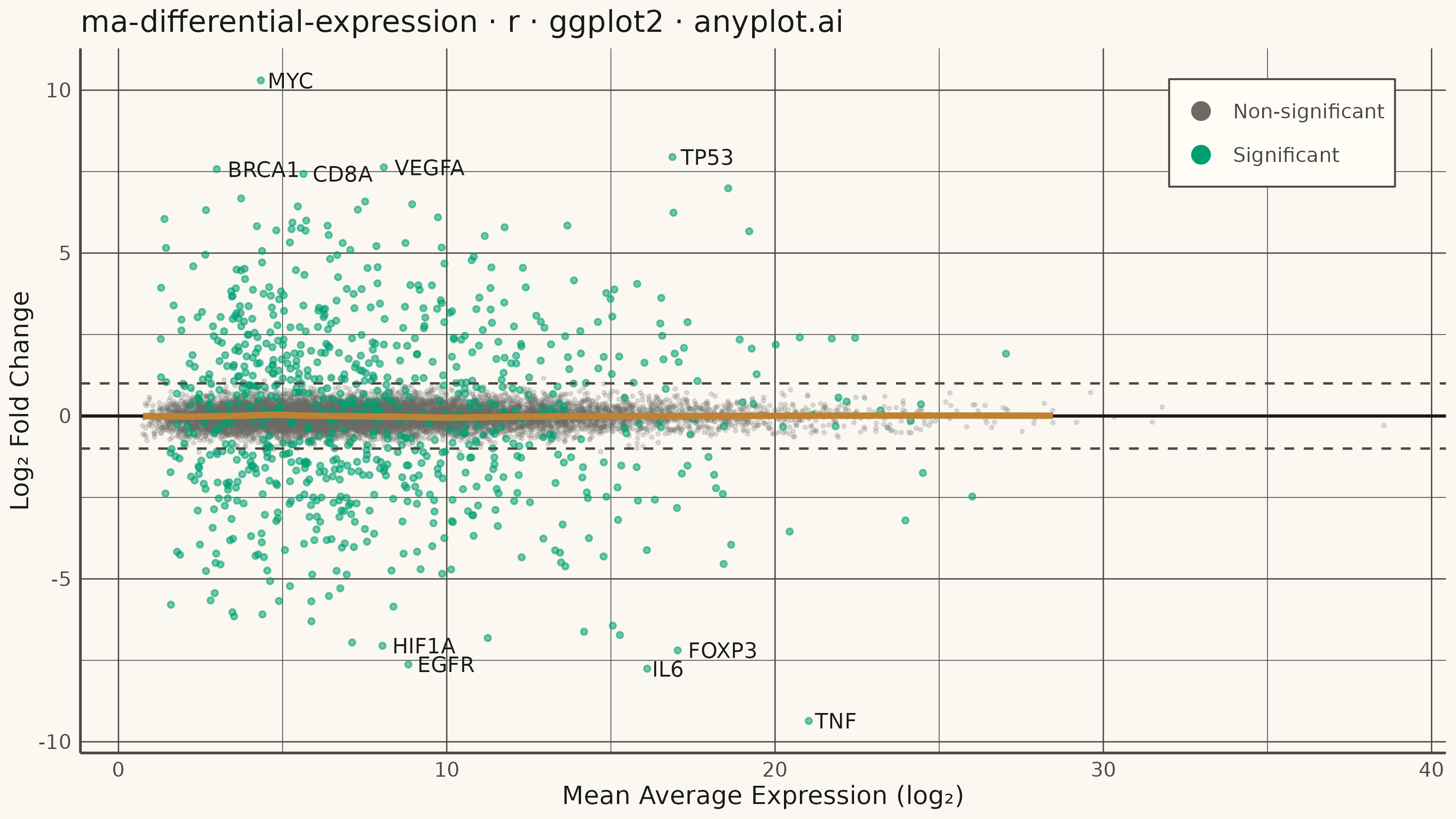
An MA plot (M-versus-A plot) visualizes the relationship between log fold change (M) and mean average expression (A) when comparing two experimental conditions. Each point represents a gene or feature, with significantly differentially expressed genes highlighted. This plot is a standard diagnostic tool in RNA-seq and microarray analysis for assessing differential expression results and detecting systematic expression-dependent bias.
#' anyplot.ai
#' ma-differential-expression: MA Plot for Differential Expression
#' Library: ggplot2 3.5.1 | R 4.4.1
#' Quality: 89/100 | Created: 2026-06-21

library(ggplot2)
library(ragg)

set.seed(42)

# Theme tokens (Imprint palette — see prompts/default-style-guide.md)
THEME       <- Sys.getenv("ANYPLOT_THEME", "light")
PAGE_BG     <- if (THEME == "light") "#FAF8F1" else "#1A1A17"
ELEVATED_BG <- if (THEME == "light") "#FFFDF6" else "#242420"
INK         <- if (THEME == "light") "#1A1A17" else "#F0EFE8"
INK_SOFT    <- if (THEME == "light") "#4A4A44" else "#B8B7B0"
INK_MUTED   <- if (THEME == "light") "#6B6A63" else "#A8A79F"

IMPRINT_PALETTE <- c(
  "#009E73",  # 1 — brand green (always first series)
  "#C475FD",  # 2 — lavender
  "#4467A3",  # 3 — blue
  "#BD8233",  # 4 — ochre
  "#AE3030",  # 5 — matte red
  "#2ABCCD",  # 6 — cyan
  "#954477",  # 7 — rose
  "#99B314"   # 8 — lime
)

# Data: simulated RNA-seq differential expression results (DESeq2-style)
n_genes  <- 12000

# A value: mean average expression (log2 baseMean), gamma-distributed for realism
mean_expr <- rgamma(n_genes, shape = 3, rate = 0.4) + 0.5

# M value: log2 fold change — centered near 0 with slight low-expression bias
lfc <- rnorm(n_genes, mean = -0.08 * exp(-mean_expr / 4), sd = 0.3)

# Significant genes (~7%): larger LFC spread
n_sig   <- round(n_genes * 0.07)
sig_idx <- sample(n_genes, n_sig)
lfc[sig_idx] <- lfc[sig_idx] + rnorm(n_sig, mean = 0, sd = 2.8)
significant <- logical(n_genes)
significant[sig_idx] <- TRUE

df <- data.frame(
  mean_expression = mean_expr,
  log_fold_change = lfc,
  significant     = significant
)

# Top 10 significant genes to label (highest |LFC|)
df_sig      <- df[df$significant, ]
df_sig_top  <- df_sig[order(abs(df_sig$log_fold_change), decreasing = TRUE), ]
top_genes   <- head(df_sig_top, 10)
top_genes$gene_name <- c("MYC", "TNF", "TP53", "IL6", "VEGFA",
                         "EGFR", "BRCA1", "CD8A", "FOXP3", "HIF1A")

# Subsample for LOESS curve (performance on large n)
df_smooth <- df[sample(nrow(df), 3000), ]

# Split for layered rendering (non-sig behind sig)
df_nonsig    <- df[!df$significant, ]
df_sig_plot  <- df[df$significant, ]

# Plot
p <- ggplot(df, aes(x = mean_expression, y = log_fold_change)) +
  # Non-significant genes
  geom_point(
    data  = df_nonsig,
    aes(color = "Non-significant"),
    alpha = 0.18,
    size  = 0.4
  ) +
  # Significant genes
  geom_point(
    data  = df_sig_plot,
    aes(color = "Significant"),
    alpha = 0.55,
    size  = 0.85
  ) +
  # Reference line at M = 0 (no change)
  geom_hline(yintercept = 0, color = INK, linewidth = 0.6) +
  # Dashed ±1 lines (2-fold change thresholds)
  geom_hline(
    yintercept = c(1, -1),
    color      = INK_SOFT,
    linewidth  = 0.45,
    linetype   = "dashed"
  ) +
  # LOESS curve to reveal expression-dependent bias
  geom_smooth(
    data        = df_smooth,
    aes(x = mean_expression, y = log_fold_change),
    method      = "loess",
    formula     = y ~ x,
    se          = FALSE,
    color       = IMPRINT_PALETTE[4],
    linewidth   = 1.2,
    span        = 0.5,
    inherit.aes = FALSE
  ) +
  # Gene labels for top differentially expressed genes
  geom_text(
    data          = top_genes,
    aes(label = gene_name),
    color         = INK,
    size          = 3.0,
    hjust         = -0.15,
    vjust         = 0.5,
    check_overlap = TRUE
  ) +
  # Color scale with legend
  scale_color_manual(
    values = c("Non-significant" = INK_MUTED, "Significant" = IMPRINT_PALETTE[1]),
    name   = NULL
  ) +
  guides(color = guide_legend(override.aes = list(size = 3, alpha = 1))) +
  labs(
    x     = "Mean Average Expression (log₂)",
    y     = "Log₂ Fold Change",
    title = "ma-differential-expression · r · ggplot2 · anyplot.ai"
  ) +
  theme_minimal(base_size = 8) +
  theme(
    plot.background   = element_rect(fill = PAGE_BG, color = PAGE_BG),
    panel.background  = element_rect(fill = PAGE_BG, color = NA),
    panel.grid.major  = element_line(color = INK_SOFT, linewidth = 0.25),
    panel.grid.minor  = element_line(color = INK_SOFT, linewidth = 0.15),
    panel.border      = element_blank(),
    axis.line         = element_line(color = INK_SOFT, linewidth = 0.5),
    axis.title        = element_text(color = INK, size = 10),
    axis.text         = element_text(color = INK_SOFT, size = 8),
    plot.title        = element_text(color = INK, size = 12),
    legend.background      = element_rect(fill = ELEVATED_BG, color = INK_SOFT),
    legend.text            = element_text(color = INK_SOFT, size = 8),
    legend.position        = "inside",
    legend.position.inside = c(0.88, 0.88)
  )

# Save
ggsave(
  filename = sprintf("plot-%s.png", THEME),
  plot     = p,
  device   = ragg::agg_png,
  width    = 8,
  height   = 4.5,
  units    = "in",
  dpi      = 400
)
Runnable source as JSON, for any HTTP client: https://api.anyplot.ai/specs/ma-differential-expression/ggplot2/code. Any spec id and library id listed in llms-full.txt fit the same URL shape; every URL below is complete and callable.
{
  "spec_id": "ma-differential-expression",
  "language": "r",
  "library": "ggplot2",
  "page": "https://anyplot.ai/ma-differential-expression/r/ggplot2",
  "hub": "https://anyplot.ai/ma-differential-expression",
  "code_json": "https://api.anyplot.ai/specs/ma-differential-expression/ggplot2/code",
  "spec_json": "https://api.anyplot.ai/specs/ma-differential-expression",
  "render_light_png": "https://storage.googleapis.com/anyplot-images/plots/ma-differential-expression/r/ggplot2/plot-light.png",
  "render_dark_png": "https://storage.googleapis.com/anyplot-images/plots/ma-differential-expression/r/ggplot2/plot-dark.png",
  "quality_score": 89.0,
  "license": "MIT",
  "guide": "https://anyplot.ai/llms.txt"
}
Part of MA Plot for Differential Expression on anyplot.ai.