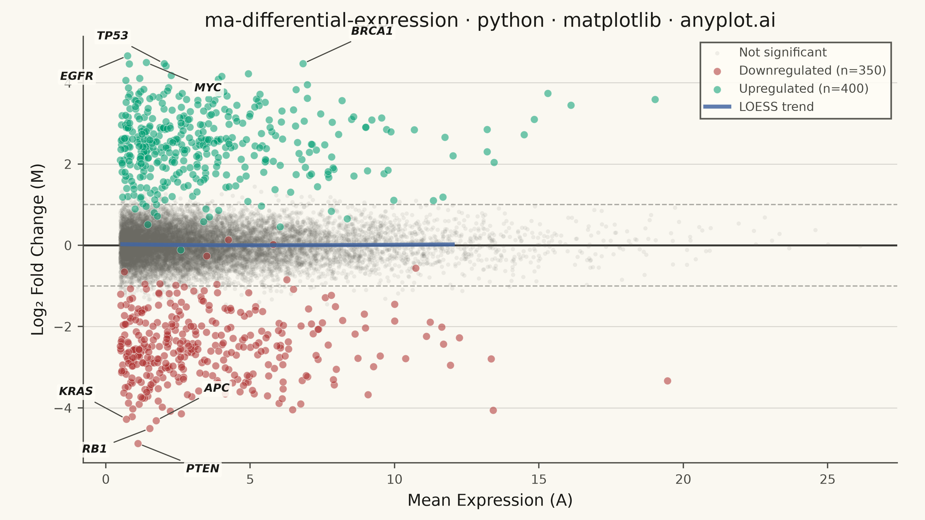
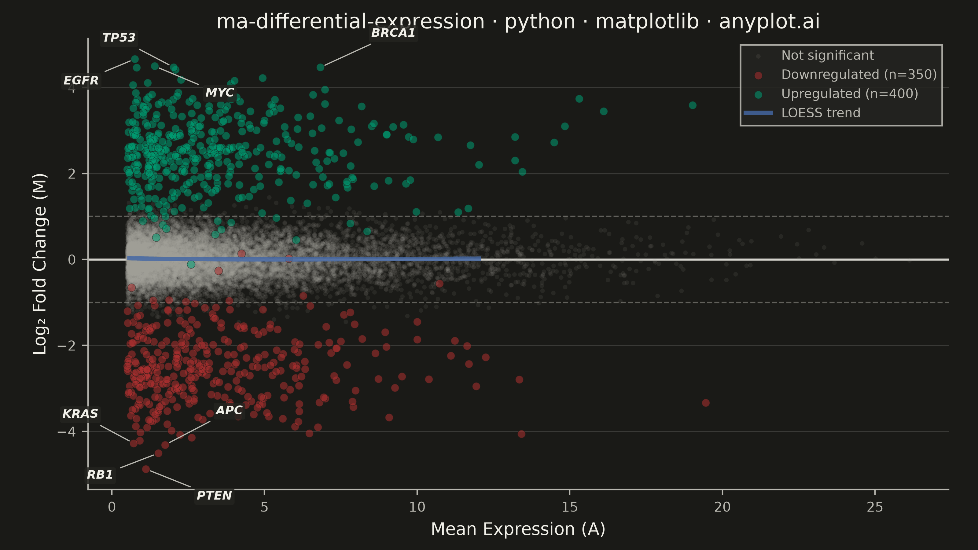
An MA plot (M-versus-A plot) visualizes the relationship between log fold change (M) and mean average expression (A) when comparing two experimental conditions. Each point represents a gene or feature, with significantly differentially expressed genes highlighted. This plot is a standard diagnostic tool in RNA-seq and microarray analysis for assessing differential expression results and detecting systematic expression-dependent bias.
""" anyplot.ai
ma-differential-expression: MA Plot for Differential Expression
Library: matplotlib 3.11.0 | Python 3.13.14
Quality: 90/100 | Updated: 2026-06-21
"""

import os
import sys


# Remove the script's own directory from sys.path so that this file (matplotlib.py)
# doesn't shadow the installed matplotlib package when run from its own directory.
_here = os.path.dirname(os.path.abspath(__file__))
sys.path = [p for p in sys.path if not p or os.path.abspath(p) != _here]

import matplotlib.pyplot as plt
import numpy as np
from scipy.interpolate import UnivariateSpline


# Theme tokens — Imprint palette (see default-style-guide.md)
THEME = os.getenv("ANYPLOT_THEME", "light")
PAGE_BG = "#FAF8F1" if THEME == "light" else "#1A1A17"
ELEVATED_BG = "#FFFDF6" if THEME == "light" else "#242420"
INK = "#1A1A17" if THEME == "light" else "#F0EFE8"
INK_SOFT = "#4A4A44" if THEME == "light" else "#B8B7B0"
INK_MUTED = "#6B6A63" if THEME == "light" else "#A8A79F"

# Imprint palette — semantic assignment for directional expression
UP_COLOR = "#009E73"  # position 1, brand green — upregulated (gain)
DOWN_COLOR = "#AE3030"  # position 5, matte red — downregulated (loss, semantic exception)
TREND_COLOR = "#4467A3"  # position 3, blue — LOESS trend line

# Data
np.random.seed(42)
n_genes = 15000

mean_expression = np.random.exponential(scale=3.0, size=n_genes) + 0.5
log_fold_change = np.random.normal(0, 0.4, size=n_genes)

n_up = 400
n_down = 350
up_idx = np.random.choice(n_genes, n_up, replace=False)
remaining = np.setdiff1d(np.arange(n_genes), up_idx)
down_idx = np.random.choice(remaining, n_down, replace=False)

log_fold_change[up_idx] = np.random.normal(2.5, 0.8, n_up)
log_fold_change[down_idx] = np.random.normal(-2.5, 0.8, n_down)

sig_mask = np.zeros(n_genes, dtype=bool)
sig_mask[up_idx] = True
sig_mask[down_idx] = True
nonsig_mask = ~sig_mask

# Top genes for labeling — alternating offsets to reduce crowding
top_up_idx = up_idx[np.argsort(log_fold_change[up_idx])[-4:]]
top_down_idx = down_idx[np.argsort(log_fold_change[down_idx])[:4]]
label_idx = np.concatenate([top_up_idx, top_down_idx])
label_names = ["BRCA1", "TP53", "MYC", "EGFR", "PTEN", "RB1", "APC", "KRAS"]
label_offsets = [
    (30, 18),
    (-42, 15),
    (30, -18),
    (-42, -15),  # upregulated: alternate right/left
    (30, -18),
    (-42, -15),
    (30, 18),
    (-42, 15),  # downregulated: alternate right/left
]

# Plot — canvas: figsize=(8, 4.5) × dpi=400 → 3200×1800 px (hard contract)
fig, ax = plt.subplots(figsize=(8, 4.5), dpi=400, facecolor=PAGE_BG)
ax.set_facecolor(PAGE_BG)

# Non-significant background cloud
ax.scatter(
    mean_expression[nonsig_mask],
    log_fold_change[nonsig_mask],
    s=7,
    alpha=0.10,
    color=INK_MUTED,
    edgecolors="none",
    rasterized=True,
    label="Not significant",
    zorder=2,
)

# Downregulated genes
ax.scatter(
    mean_expression[down_idx],
    log_fold_change[down_idx],
    s=22,
    alpha=0.55,
    color=DOWN_COLOR,
    edgecolors=PAGE_BG,
    linewidth=0.3,
    rasterized=True,
    label=f"Downregulated (n={n_down})",
    zorder=3,
)

# Upregulated genes
ax.scatter(
    mean_expression[up_idx],
    log_fold_change[up_idx],
    s=22,
    alpha=0.55,
    color=UP_COLOR,
    edgecolors=PAGE_BG,
    linewidth=0.3,
    rasterized=True,
    label=f"Upregulated (n={n_up})",
    zorder=3,
)

# Reference lines
ax.axhline(y=0, color=INK, linewidth=1.2, alpha=0.85, zorder=1)
ax.axhline(y=1, color=INK_SOFT, linewidth=0.8, linestyle="--", alpha=0.45, zorder=1)
ax.axhline(y=-1, color=INK_SOFT, linewidth=0.8, linestyle="--", alpha=0.45, zorder=1)

# LOESS trend — binned spline approximation over all genes
sorted_idx = np.argsort(mean_expression)
x_sorted = mean_expression[sorted_idx]
y_sorted = log_fold_change[sorted_idx]

bin_count = 80
bin_edges = np.linspace(x_sorted.min(), np.percentile(x_sorted, 98), bin_count + 1)
bin_centers, bin_means = [], []
for i in range(bin_count):
    in_bin = (x_sorted >= bin_edges[i]) & (x_sorted < bin_edges[i + 1])
    if in_bin.sum() > 10:
        bin_centers.append((bin_edges[i] + bin_edges[i + 1]) / 2)
        bin_means.append(np.mean(y_sorted[in_bin]))

bin_centers = np.array(bin_centers)
bin_means = np.array(bin_means)
spline = UnivariateSpline(bin_centers, bin_means, s=len(bin_centers) * 0.5)
x_smooth = np.linspace(bin_centers.min(), bin_centers.max(), 200)
y_smooth = spline(x_smooth)
ax.plot(x_smooth, y_smooth, color=TREND_COLOR, linewidth=2.5, alpha=0.85, label="LOESS trend", zorder=4)

# Gene annotations with connector arrows (arrowprops) and background bbox for readability
for gene_idx, name, (dx, dy) in zip(label_idx, label_names, label_offsets, strict=False):
    ax.annotate(
        name,
        xy=(mean_expression[gene_idx], log_fold_change[gene_idx]),
        xytext=(dx, dy),
        textcoords="offset points",
        fontsize=7,
        fontweight="bold",
        fontstyle="italic",
        color=INK,
        bbox={"facecolor": ELEVATED_BG, "edgecolor": "none", "alpha": 0.85, "pad": 1.5, "boxstyle": "round,pad=0.2"},
        arrowprops={"arrowstyle": "-", "color": INK_SOFT, "linewidth": 0.7, "shrinkA": 3, "shrinkB": 3},
        zorder=5,
    )

# Style — font sizes per library guide (3200×1800 canvas)
title = "ma-differential-expression · python · matplotlib · anyplot.ai"
ax.set_xlabel("Mean Expression (A)", fontsize=10, color=INK)
ax.set_ylabel("Log₂ Fold Change (M)", fontsize=10, color=INK)
ax.set_title(title, fontsize=12, fontweight="medium", color=INK)
ax.tick_params(axis="both", labelsize=8, colors=INK_SOFT)
ax.spines["top"].set_visible(False)
ax.spines["right"].set_visible(False)
ax.spines["left"].set_color(INK_SOFT)
ax.spines["bottom"].set_color(INK_SOFT)
ax.yaxis.grid(True, alpha=0.15, linewidth=0.6, color=INK)

leg = ax.legend(fontsize=7.5, loc="upper right", framealpha=0.9, edgecolor=INK_SOFT, fancybox=False)
if leg:
    leg.get_frame().set_facecolor(ELEVATED_BG)
    plt.setp(leg.get_texts(), color=INK_SOFT)

fig.subplots_adjust(left=0.09, right=0.97, top=0.93, bottom=0.11)

# Save — bbox_inches must stay default (None) to preserve 3200×1800 canvas
plt.savefig(f"plot-{THEME}.png", dpi=400, facecolor=PAGE_BG)
plt.close()
Runnable source as JSON, for any HTTP client: https://api.anyplot.ai/specs/ma-differential-expression/matplotlib/code. Any spec id and library id listed in llms-full.txt fit the same URL shape; every URL below is complete and callable.
{
  "spec_id": "ma-differential-expression",
  "language": "python",
  "library": "matplotlib",
  "page": "https://anyplot.ai/ma-differential-expression/python/matplotlib",
  "hub": "https://anyplot.ai/ma-differential-expression",
  "code_json": "https://api.anyplot.ai/specs/ma-differential-expression/matplotlib/code",
  "spec_json": "https://api.anyplot.ai/specs/ma-differential-expression",
  "render_light_png": "https://storage.googleapis.com/anyplot-images/plots/ma-differential-expression/python/matplotlib/plot-light.png",
  "render_dark_png": "https://storage.googleapis.com/anyplot-images/plots/ma-differential-expression/python/matplotlib/plot-dark.png",
  "quality_score": 90.0,
  "license": "MIT",
  "guide": "https://anyplot.ai/llms.txt"
}
Part of MA Plot for Differential Expression on anyplot.ai.