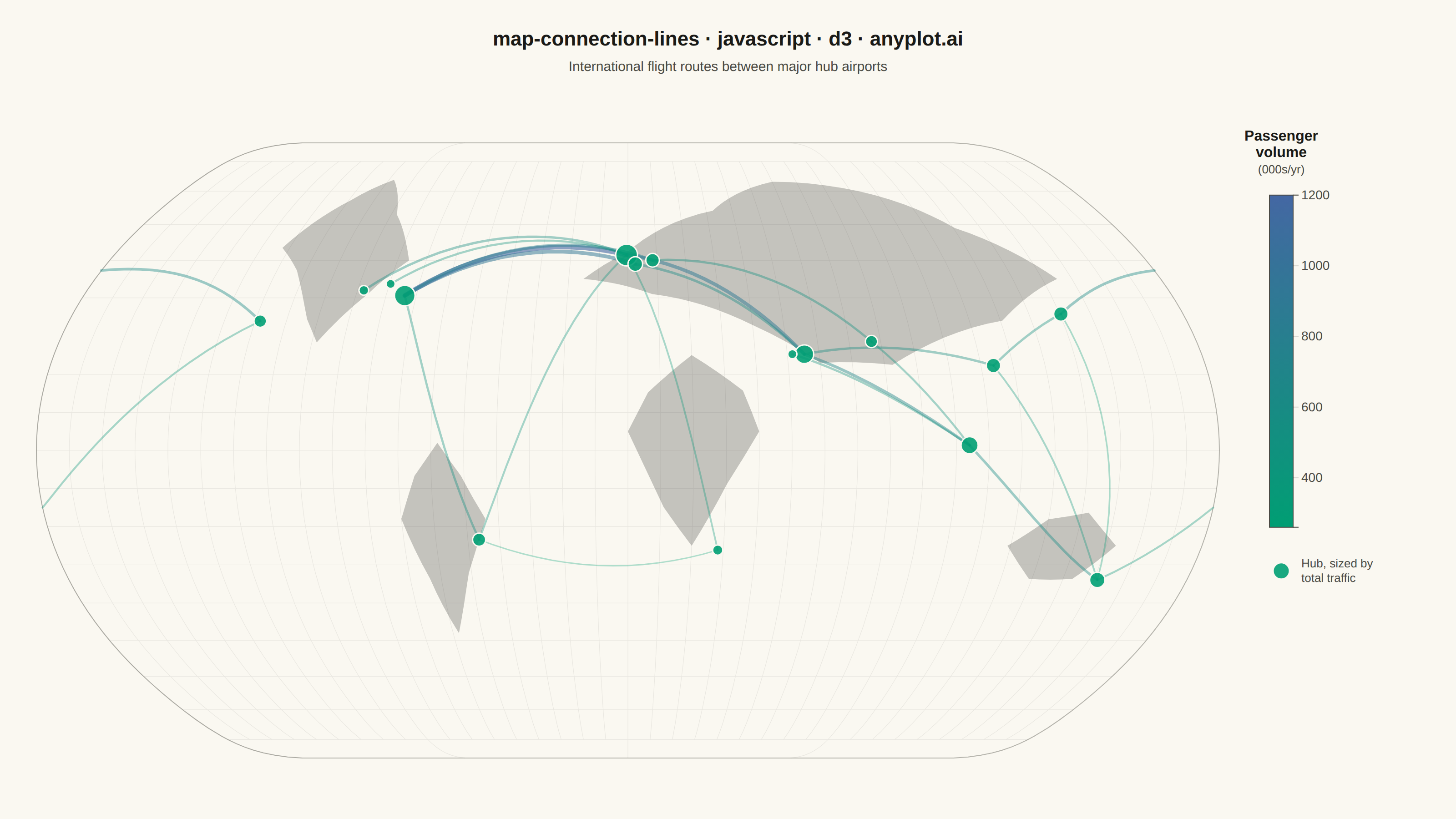
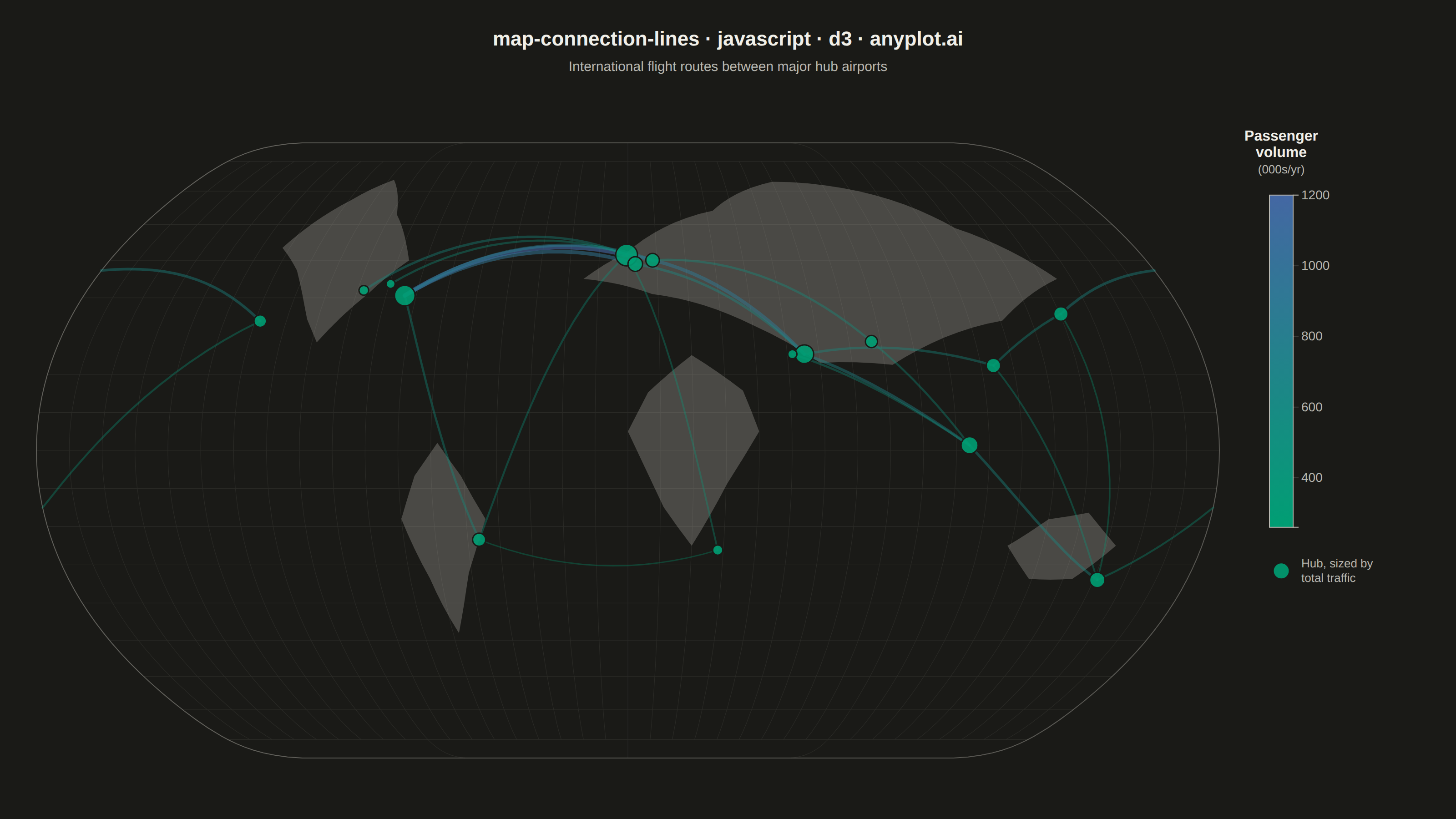
The same plot in 14 other libraries — JavaScript: Chart.js, Apache ECharts, Highcharts, MUI X Charts; Python: Altair, Bokeh, lets-plot, Matplotlib, Plotly, plotnine, Pygal, Seaborn; R: ggplot2; Julia: Makie.jl. Compare all 15 side by side: Connection Lines Map (Origin-Destination) in Python, R, Julia and JavaScript.
A geographic map visualization showing connection lines (arcs or great circles) between pairs of locations. This plot excels at revealing spatial patterns in flows, routes, and relationships between places. The curved lines naturally represent shortest paths on Earth's surface while avoiding visual overlap with straight lines. Line properties like thickness or color can encode additional variables such as traffic volume or connection type.
// anyplot.ai
// map-connection-lines: Connection Lines Map (Origin-Destination)
// Library: d3 7.9.0 | JavaScript 22.23.2
// Quality: 88/100 | Created: 2026-08-26

const t = window.ANYPLOT_TOKENS;
const { width, height } = window.ANYPLOT_SIZE;

// --- Data: international flight routes between major hub airports ----------
const hubs = [
  { id: "JFK", name: "New York", lon: -73.8, lat: 40.6 },
  { id: "LAX", name: "Los Angeles", lon: -118.4, lat: 33.9 },
  { id: "ORD", name: "Chicago", lon: -87.9, lat: 41.98 },
  { id: "YYZ", name: "Toronto", lon: -79.63, lat: 43.68 },
  { id: "GRU", name: "Sao Paulo", lon: -46.47, lat: -23.43 },
  { id: "LHR", name: "London", lon: -0.45, lat: 51.47 },
  { id: "CDG", name: "Paris", lon: 2.55, lat: 49.0 },
  { id: "FRA", name: "Frankfurt", lon: 8.57, lat: 50.03 },
  { id: "JNB", name: "Johannesburg", lon: 28.25, lat: -26.13 },
  { id: "DXB", name: "Dubai", lon: 55.36, lat: 25.25 },
  { id: "DOH", name: "Doha", lon: 51.6, lat: 25.27 },
  { id: "DEL", name: "Delhi", lon: 77.1, lat: 28.56 },
  { id: "SIN", name: "Singapore", lon: 103.99, lat: 1.36 },
  { id: "HKG", name: "Hong Kong", lon: 113.9, lat: 22.3 },
  { id: "NRT", name: "Tokyo", lon: 140.39, lat: 35.76 },
  { id: "SYD", name: "Sydney", lon: 151.18, lat: -33.95 },
];
const hubById = new Map(hubs.map((h) => [h.id, h]));

// value: annual passenger volume, thousands
const routes = [
  { from: "JFK", to: "LHR", value: 1200 },
  { from: "JFK", to: "CDG", value: 950 },
  { from: "JFK", to: "FRA", value: 780 },
  { from: "LAX", to: "NRT", value: 640 },
  { from: "LAX", to: "SYD", value: 420 },
  { from: "LHR", to: "DXB", value: 890 },
  { from: "LHR", to: "JNB", value: 380 },
  { from: "CDG", to: "DXB", value: 610 },
  { from: "FRA", to: "DEL", value: 520 },
  { from: "DXB", to: "SIN", value: 700 },
  { from: "DXB", to: "HKG", value: 560 },
  { from: "DOH", to: "SIN", value: 480 },
  { from: "SIN", to: "SYD", value: 610 },
  { from: "HKG", to: "NRT", value: 540 },
  { from: "HKG", to: "SYD", value: 390 },
  { from: "DEL", to: "SIN", value: 460 },
  { from: "GRU", to: "JNB", value: 260 },
  { from: "GRU", to: "LHR", value: 430 },
  { from: "ORD", to: "LHR", value: 560 },
  { from: "YYZ", to: "LHR", value: 470 },
  { from: "JFK", to: "GRU", value: 500 },
  { from: "NRT", to: "SYD", value: 330 },
];

const nodeTotals = new Map();
for (const r of routes) {
  nodeTotals.set(r.from, (nodeTotals.get(r.from) || 0) + r.value);
  nodeTotals.set(r.to, (nodeTotals.get(r.to) || 0) + r.value);
}

// --- Layout ------------------------------------------------------------
const margin = { top: 130, right: 260, bottom: 40, left: 40 };
const mapW = width - margin.left - margin.right;
const mapH = height - margin.top - margin.bottom;

// --- Projection: whole-world pseudo-cylindrical, fit to the map area -------
const projection = d3.geoNaturalEarth1().fitExtent(
  [
    [0, 0],
    [mapW, mapH],
  ],
  { type: "Sphere" },
);
projection.precision(0.15); // finer resampling so great-circle arcs read smoothly
const path = d3.geoPath(projection);
const graticule = d3.geoGraticule10();

// --- Scales --------------------------------------------------------------
const valueExtent = d3.extent(routes, (d) => d.value);
const arcColor = d3.scaleSequential(d3.interpolateRgbBasis(t.seq)).domain(valueExtent);
const arcWidth = d3.scaleLinear().domain(valueExtent).range([1.5, 5]);
const arcOpacity = d3.scaleLinear().domain(valueExtent).range([0.3, 0.6]);
const nodeRadius = d3
  .scaleSqrt()
  .domain(d3.extent(Array.from(nodeTotals.values())))
  .range([5, 12]);

// --- SVG mount -----------------------------------------------------------
const svg = d3.select("#container").append("svg").attr("width", width).attr("height", height);
const g = svg.append("g").attr("transform", `translate(${margin.left},${margin.top})`);
const mapG = g.append("g");

// Sphere outline — the globe's silhouette under the Natural Earth projection
mapG
  .append("path")
  .datum({ type: "Sphere" })
  .attr("d", path)
  .attr("fill", "none")
  .attr("stroke", t.inkSoft)
  .attr("stroke-width", 1)
  .attr("stroke-opacity", 0.4);

// Graticule — subtle lon/lat grid for geographic context
mapG
  .append("path")
  .datum(graticule)
  .attr("d", path)
  .attr("fill", "none")
  .attr("stroke", t.grid)
  .attr("stroke-width", 0.6)
  .attr("stroke-opacity", 0.5);

// Simplified continent silhouettes — abstract, non-self-intersecting blobs for
// geographic context (not political borders). Built from a center plus radii
// sampled at strictly increasing angles, which guarantees a simple polygon.
// d3-geo's spherical winding rule is the opposite of planar-SVG intuition: a
// ring built by increasing angle (counterclockwise in the standard lon/lat
// plane) is interpreted as the *complement* — the whole sphere minus the
// blob — so each "continent" ends up covering almost the entire globe
// instead of a small patch. Reversing the ring flips it back to the small
// enclosed area that was actually intended.
function blobRing(clon, clat, radii) {
  const ring = radii.map(([angleDeg, rLon, rLat]) => {
    const rad = (angleDeg * Math.PI) / 180;
    return [clon + rLon * Math.cos(rad), clat + rLat * Math.sin(rad)];
  });
  ring.reverse();
  ring.push(ring[0]);
  return ring;
}

const continents = [
  {
    name: "North America",
    coordinates: blobRing(-100, 50, [
      [0, 24, 8], [40, 16, 20], [80, 12, 24], [120, 18, 20], [160, 24, 10],
      [200, 14, 8], [240, 7, 18], [280, 9, 22], [320, 18, 14],
    ]),
  },
  {
    name: "South America",
    coordinates: blobRing(-58, -18, [
      [0, 14, 10], [45, 10, 16], [90, 8, 20], [135, 10, 16], [180, 12, 10],
      [225, 8, 22], [270, 6, 30], [315, 10, 20],
    ]),
  },
  {
    name: "Africa",
    coordinates: blobRing(20, 5, [
      [0, 20, 10], [50, 24, 14], [90, 14, 20], [140, 18, 16], [180, 20, 10],
      [230, 14, 26], [270, 10, 30], [310, 16, 18],
    ]),
  },
  {
    name: "Eurasia",
    coordinates: blobRing(60, 45, [
      [0, 85, 20], [30, 70, 28], [60, 55, 30], [90, 40, 28], [120, 55, 22],
      [150, 70, 14], [180, 75, 10], [210, 60, 8], [240, 40, 14], [270, 30, 22],
      [300, 45, 26], [330, 70, 22],
    ]),
  },
  {
    name: "Australia",
    coordinates: blobRing(135, -25, [
      [0, 18, 8], [60, 14, 10], [120, 10, 8], [180, 16, 8], [240, 12, 10],
      [300, 16, 10],
    ]),
  },
];

// Note: ANYPLOT_TOKENS has no `muted` key (only pageBg/elevatedBg/ink/inkSoft/
// grid/palette/amber/seq/div) — using it here would leave `fill` unset, and the
// SVG UA-default fill is solid black, which is what caused the map interior to
// render as a near-black disc regardless of theme. `t.inkSoft` is the defined,
// theme-adaptive token closest to the intended "muted neutral" role.
mapG
  .selectAll("path.landmass")
  .data(continents)
  .join("path")
  .attr("class", "landmass")
  .attr("d", (d) => path({ type: "Polygon", coordinates: [d.coordinates] }))
  .attr("fill", t.inkSoft)
  .attr("fill-opacity", 0.3)
  .attr("stroke", "none");

// Tooltip — real hover, only live in the exported interactive HTML
const tooltip = d3
  .select("#container")
  .append("div")
  .style("position", "fixed")
  .style("pointer-events", "none")
  .style("opacity", 0)
  .style("background", t.elevatedBg)
  .style("color", t.ink)
  .style("border", `1px solid ${t.grid}`)
  .style("border-radius", "6px")
  .style("padding", "8px 10px")
  .style("font-size", "13px")
  .style("font-family", "sans-serif")
  .style("line-height", "1.5")
  .style("box-shadow", "0 2px 8px rgba(0,0,0,0.25)")
  .style("transition", "opacity 0.1s linear");

// Connection arcs — geodesic (great-circle) paths, thickness + color encode
// passenger volume; d3.geoPath adaptively resamples a 2-point LineString
// along the sphere, so this bows the way a real flight route would.
mapG
  .selectAll("path.route")
  .data(routes)
  .join("path")
  .attr("class", "route")
  .attr("d", (d) => {
    const o = hubById.get(d.from);
    const e = hubById.get(d.to);
    return path({
      type: "LineString",
      coordinates: [
        [o.lon, o.lat],
        [e.lon, e.lat],
      ],
    });
  })
  .attr("fill", "none")
  .attr("stroke", (d) => arcColor(d.value))
  .attr("stroke-width", (d) => arcWidth(d.value))
  .attr("stroke-opacity", (d) => arcOpacity(d.value))
  .attr("stroke-linecap", "round")
  .style("cursor", "pointer")
  .on("mouseenter", function (event, d) {
    d3.select(this).attr("stroke-opacity", 1);
    tooltip.style("opacity", 1);
  })
  .on("mousemove", function (event, d) {
    const o = hubById.get(d.from);
    const e = hubById.get(d.to);
    tooltip
      .style("left", `${event.clientX + 16}px`)
      .style("top", `${event.clientY + 16}px`)
      .html(`<strong>${o.name} → ${e.name}</strong><br>${d.value}k passengers/yr`);
  })
  .on("mouseleave", function (event, d) {
    d3.select(this).attr("stroke-opacity", arcOpacity(d.value));
    tooltip.style("opacity", 0);
  });

// Hub markers — location endpoints, sized by total connected volume
mapG
  .selectAll("circle.hub")
  .data(hubs)
  .join("circle")
  .attr("class", "hub")
  .attr("cx", (d) => projection([d.lon, d.lat])[0])
  .attr("cy", (d) => projection([d.lon, d.lat])[1])
  .attr("r", (d) => nodeRadius(nodeTotals.get(d.id) || 0))
  .attr("fill", t.palette[0])
  .attr("fill-opacity", 0.9)
  .attr("stroke", t.pageBg)
  .attr("stroke-width", 1.5)
  .style("cursor", "pointer")
  .on("mouseenter", function () {
    d3.select(this).attr("stroke", t.ink);
    tooltip.style("opacity", 1);
  })
  .on("mousemove", function (event, d) {
    tooltip
      .style("left", `${event.clientX + 16}px`)
      .style("top", `${event.clientY + 16}px`)
      .html(`<strong>${d.name}</strong><br>${nodeTotals.get(d.id)}k connected passengers/yr`);
  })
  .on("mouseleave", function () {
    d3.select(this).attr("stroke", t.pageBg);
    tooltip.style("opacity", 0);
  });

// --- Legend: passenger volume (color + width) -----------------------------
const legendW = 26;
const legendH = mapH * 0.5;
const legendX = mapW + 55;
const legendY = mapH * 0.08;
const nStops = 10;

svg
  .append("defs")
  .append("linearGradient")
  .attr("id", "legend-gradient")
  .attr("x1", "0%")
  .attr("y1", "100%")
  .attr("x2", "0%")
  .attr("y2", "0%")
  .selectAll("stop")
  .data(d3.range(nStops + 1))
  .join("stop")
  .attr("offset", (d) => `${(d / nStops) * 100}%`)
  .attr("stop-color", (d) => arcColor(valueExtent[0] + (d / nStops) * (valueExtent[1] - valueExtent[0])));

const legendG = g.append("g").attr("transform", `translate(${legendX},${legendY})`);
const legendRectTop = 26; // clears the title/unit text stacked above the bar
legendG
  .append("rect")
  .attr("y", legendRectTop)
  .attr("width", legendW)
  .attr("height", legendH)
  .attr("fill", "url(#legend-gradient)")
  .attr("stroke", t.inkSoft)
  .attr("stroke-width", 1);

const legendScale = d3.scaleLinear().domain(valueExtent).range([legendH + legendRectTop, legendRectTop]);
const legendAxis = d3
  .axisRight(legendScale)
  .ticks(5)
  .tickFormat((d) => d.toFixed(0));
const legendAxisG = legendG.append("g").attr("transform", `translate(${legendW},0)`).call(legendAxis);
legendAxisG.selectAll("text").attr("fill", t.inkSoft).style("font-size", "14px");
legendAxisG.selectAll("line").attr("stroke", t.grid);
legendAxisG.select(".domain").attr("stroke", t.inkSoft);

legendG
  .append("text")
  .attr("x", legendW / 2)
  .attr("y", -34)
  .attr("text-anchor", "middle")
  .attr("fill", t.ink)
  .style("font-size", "16px")
  .style("font-weight", "600")
  .text("Passenger");

legendG
  .append("text")
  .attr("x", legendW / 2)
  .attr("y", -16)
  .attr("text-anchor", "middle")
  .attr("fill", t.ink)
  .style("font-size", "16px")
  .style("font-weight", "600")
  .text("volume");

legendG
  .append("text")
  .attr("x", legendW / 2)
  .attr("y", 2)
  .attr("text-anchor", "middle")
  .attr("fill", t.inkSoft)
  .style("font-size", "13px")
  .text("(000s/yr)");

// Marker-size note, placed under the volume legend for context
legendG
  .append("circle")
  .attr("cx", legendW / 2)
  .attr("cy", legendH + legendRectTop + 48)
  .attr("r", 9)
  .attr("fill", t.palette[0])
  .attr("fill-opacity", 0.9)
  .attr("stroke", t.pageBg)
  .attr("stroke-width", 1.5);
legendG
  .append("text")
  .attr("x", legendW / 2 + 22)
  .attr("y", legendH + legendRectTop + 44)
  .attr("fill", t.inkSoft)
  .style("font-size", "13px")
  .text("Hub, sized by");
legendG
  .append("text")
  .attr("x", legendW / 2 + 22)
  .attr("y", legendH + legendRectTop + 60)
  .attr("fill", t.inkSoft)
  .style("font-size", "13px")
  .text("total traffic");

// --- Title -----------------------------------------------------------------
svg
  .append("text")
  .attr("x", width / 2)
  .attr("y", 50)
  .attr("text-anchor", "middle")
  .attr("fill", t.ink)
  .style("font-size", "22px")
  .style("font-weight", "600")
  .text("map-connection-lines · javascript · d3 · anyplot.ai");

svg
  .append("text")
  .attr("x", width / 2)
  .attr("y", 78)
  .attr("text-anchor", "middle")
  .attr("fill", t.inkSoft)
  .style("font-size", "15px")
  .text("International flight routes between major hub airports");
Runnable source as JSON, for any HTTP client: https://api.anyplot.ai/specs/map-connection-lines/d3/code. Any spec id and library id listed in llms-full.txt fit the same URL shape; every URL below is complete and callable.
{
  "spec_id": "map-connection-lines",
  "language": "javascript",
  "library": "d3",
  "page": "https://anyplot.ai/map-connection-lines/javascript/d3",
  "hub": "https://anyplot.ai/map-connection-lines",
  "code_json": "https://api.anyplot.ai/specs/map-connection-lines/d3/code",
  "spec_json": "https://api.anyplot.ai/specs/map-connection-lines",
  "render_light_png": "https://storage.googleapis.com/anyplot-images/plots/map-connection-lines/javascript/d3/plot-light.png",
  "render_dark_png": "https://storage.googleapis.com/anyplot-images/plots/map-connection-lines/javascript/d3/plot-dark.png",
  "interactive_light_html": "https://storage.googleapis.com/anyplot-images/plots/map-connection-lines/javascript/d3/plot-light.html",
  "interactive_dark_html": "https://storage.googleapis.com/anyplot-images/plots/map-connection-lines/javascript/d3/plot-dark.html",
  "quality_score": 88.0,
  "license": "MIT",
  "guide": "https://anyplot.ai/llms.txt"
}
Part of Connection Lines Map (Origin-Destination) on anyplot.ai.