The same plot in 14 other libraries — Python: Bokeh, lets-plot, Matplotlib, Plotly, plotnine, Pygal, Seaborn; R: ggplot2; Julia: Makie.jl; JavaScript: Chart.js, D3.js, Apache ECharts, Highcharts, MUI X Charts. Compare all 15 side by side: Connection Lines Map (Origin-Destination) in Python, R, Julia and JavaScript.
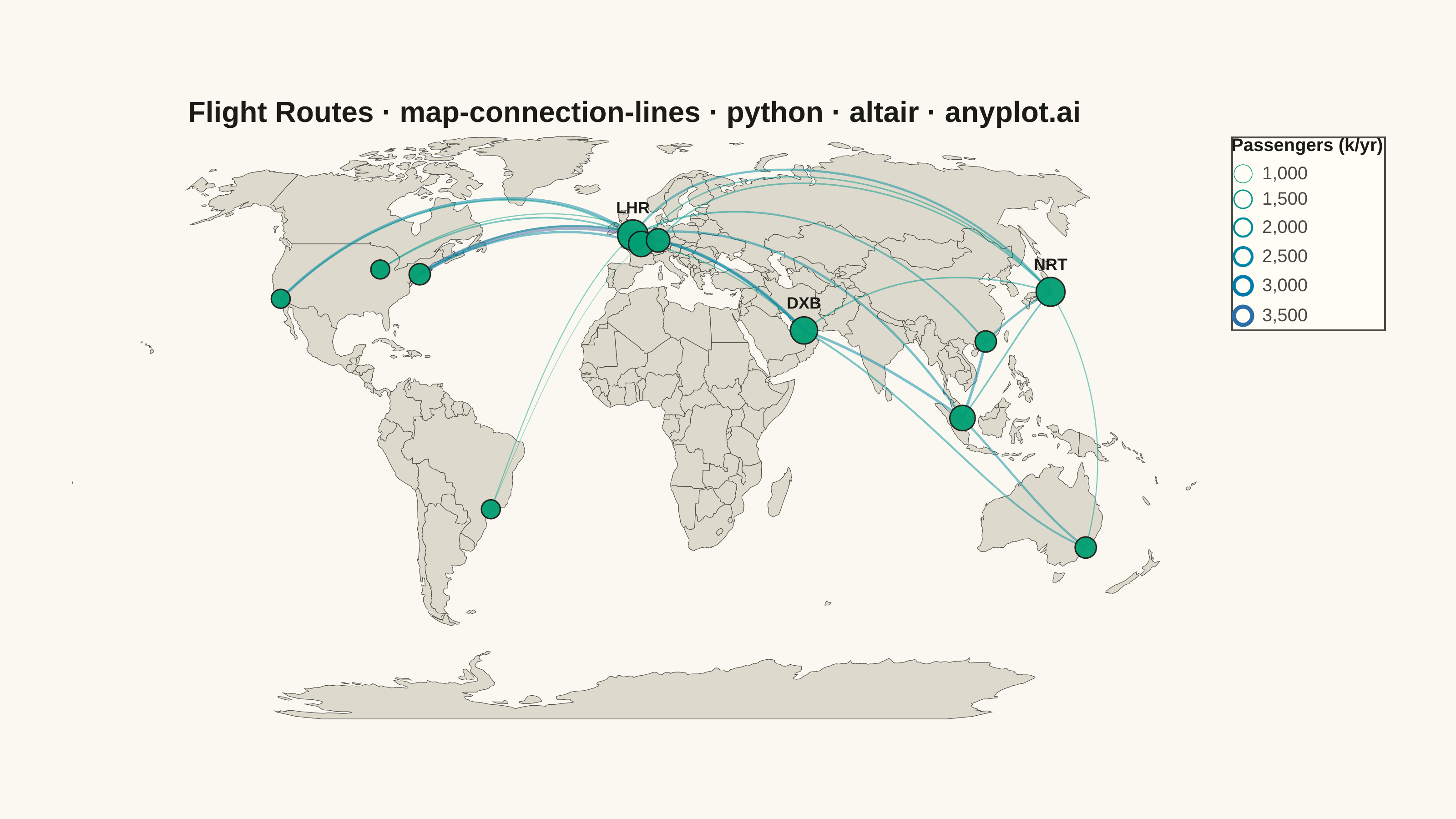
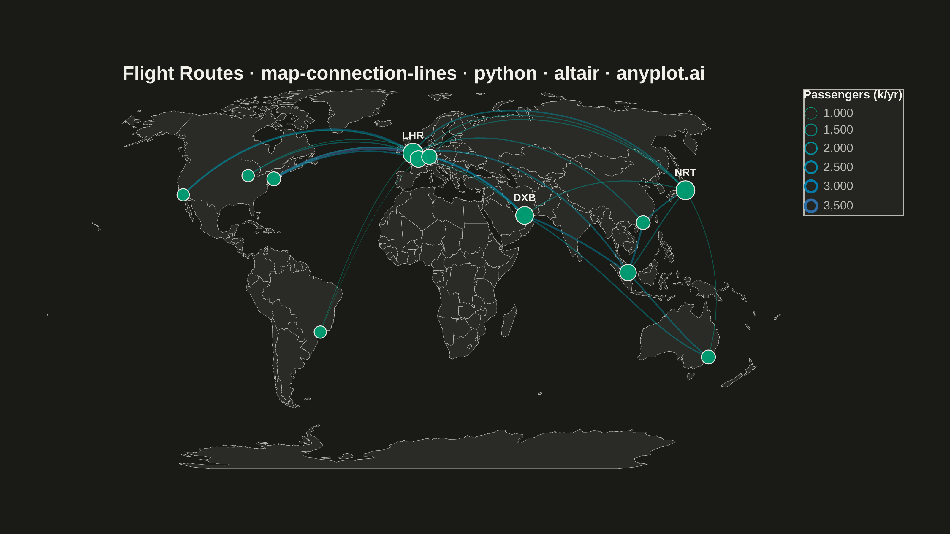
A geographic map visualization showing connection lines (arcs or great circles) between pairs of locations. This plot excels at revealing spatial patterns in flows, routes, and relationships between places. The curved lines naturally represent shortest paths on Earth's surface while avoiding visual overlap with straight lines. Line properties like thickness or color can encode additional variables such as traffic volume or connection type.
""" anyplot.ai
map-connection-lines: Connection Lines Map (Origin-Destination)
Library: altair 6.1.0 | Python 3.13.13
Quality: 92/100 | Created: 2026-05-28
"""

import os
import sys
from collections import Counter


# Prevent self-import: this file is named altair.py, so we must remove its
# directory from sys.path before importing the altair package.
_this_dir = os.path.dirname(os.path.abspath(__file__))
sys.path = [p for p in sys.path if p and os.path.abspath(p) != _this_dir]

import altair as alt
import numpy as np
import pandas as pd
from PIL import Image


# Theme tokens
THEME = os.getenv("ANYPLOT_THEME", "light")
PAGE_BG = "#FAF8F1" if THEME == "light" else "#1A1A17"
ELEVATED_BG = "#FFFDF6" if THEME == "light" else "#242420"
INK = "#1A1A17" if THEME == "light" else "#F0EFE8"
INK_SOFT = "#4A4A44" if THEME == "light" else "#B8B7B0"
MAP_LAND = "#DDD9CC" if THEME == "light" else "#2A2A26"
PAGE_BG_TUPLE = (250, 248, 241) if THEME == "light" else (26, 26, 23)

BRAND = "#009E73"

# Data: major airports (avoiding trans-Pacific routes that cross the antimeridian)
airports = {
    "JFK": {"lat": 40.6, "lon": -73.8, "city": "New York"},
    "LAX": {"lat": 33.9, "lon": -118.4, "city": "Los Angeles"},
    "ORD": {"lat": 41.9, "lon": -87.9, "city": "Chicago"},
    "GRU": {"lat": -23.5, "lon": -46.6, "city": "Sao Paulo"},
    "LHR": {"lat": 51.5, "lon": -0.5, "city": "London"},
    "CDG": {"lat": 49.0, "lon": 2.5, "city": "Paris"},
    "FRA": {"lat": 50.0, "lon": 8.6, "city": "Frankfurt"},
    "DXB": {"lat": 25.3, "lon": 55.4, "city": "Dubai"},
    "SIN": {"lat": 1.4, "lon": 103.9, "city": "Singapore"},
    "HKG": {"lat": 22.3, "lon": 113.9, "city": "Hong Kong"},
    "NRT": {"lat": 35.8, "lon": 140.4, "city": "Tokyo"},
    "SYD": {"lat": -33.9, "lon": 151.2, "city": "Sydney"},
}

# Flight routes (origin, destination, annual passengers in thousands)
routes_raw = [
    ("JFK", "LHR", 3800),
    ("JFK", "CDG", 2200),
    ("JFK", "FRA", 1900),
    ("LAX", "LHR", 2600),
    ("LAX", "CDG", 1600),
    ("ORD", "LHR", 1700),
    ("ORD", "FRA", 1300),
    ("GRU", "LHR", 1200),
    ("GRU", "CDG", 900),
    ("LHR", "DXB", 2900),
    ("CDG", "DXB", 1400),
    ("FRA", "DXB", 2200),
    ("DXB", "SIN", 2400),
    ("DXB", "SYD", 1900),
    ("DXB", "NRT", 1600),
    ("LHR", "SIN", 2200),
    ("LHR", "HKG", 1800),
    ("LHR", "NRT", 2100),
    ("FRA", "NRT", 1600),
    ("CDG", "NRT", 1500),
    ("NRT", "SIN", 1700),
    ("NRT", "HKG", 2100),
    ("NRT", "SYD", 1300),
    ("SIN", "SYD", 2100),
    ("HKG", "SIN", 2500),
]

# Hub connectivity: count routes per airport
connectivity = Counter()
for origin, dest, _ in routes_raw:
    connectivity[origin] += 1
    connectivity[dest] += 1

# Generate great circle arc points via spherical linear interpolation (SLERP)
n_arc_points = 40
arc_records = []
for origin_code, dest_code, volume in routes_raw:
    olat = airports[origin_code]["lat"]
    olon = airports[origin_code]["lon"]
    dlat = airports[dest_code]["lat"]
    dlon = airports[dest_code]["lon"]

    lat1_r = np.radians(olat)
    lon1_r = np.radians(olon)
    lat2_r = np.radians(dlat)
    lon2_r = np.radians(dlon)

    x1 = np.cos(lat1_r) * np.cos(lon1_r)
    y1 = np.cos(lat1_r) * np.sin(lon1_r)
    z1 = np.sin(lat1_r)

    x2 = np.cos(lat2_r) * np.cos(lon2_r)
    y2 = np.cos(lat2_r) * np.sin(lon2_r)
    z2 = np.sin(lat2_r)

    dot = float(np.clip(x1 * x2 + y1 * y2 + z1 * z2, -1, 1))
    omega = np.arccos(dot)

    for j, t in enumerate(np.linspace(0, 1, n_arc_points)):
        if omega < 1e-10:
            pt_lat, pt_lon = olat, olon
        else:
            sin_omega = np.sin(omega)
            a = np.sin((1 - t) * omega) / sin_omega
            b = np.sin(t * omega) / sin_omega
            x = a * x1 + b * x2
            y = a * y1 + b * y2
            z = a * z1 + b * z2
            pt_lat = float(np.degrees(np.arctan2(z, np.sqrt(x**2 + y**2))))
            pt_lon = float(np.degrees(np.arctan2(y, x)))

        arc_records.append(
            {
                "latitude": pt_lat,
                "longitude": pt_lon,
                "route": f"{origin_code}-{dest_code}",
                "volume": volume,
                "order": j,
            }
        )

arcs_df = pd.DataFrame(arc_records)

# Airport markers dataframe with connectivity for size scaling
airports_df = pd.DataFrame(
    [
        {
            "code": code,
            "city": info["city"],
            "latitude": info["lat"],
            "longitude": info["lon"],
            "connections": connectivity[code],
        }
        for code, info in airports.items()
    ]
)

# Title (67 chars → fontSize=16, no scaling needed)
title_str = "Flight Routes · map-connection-lines · python · altair · anyplot.ai"
n_chars = len(title_str)
title_fs = round(16 * 67 / n_chars) if n_chars > 67 else 16

# World map base layer (110m resolution topojson)
world_url = "https://cdn.jsdelivr.net/npm/vega-datasets@2/data/world-110m.json"

base_map = alt.Chart(alt.topo_feature(world_url, "countries")).mark_geoshape(
    fill=MAP_LAND, stroke=INK_SOFT, strokeWidth=0.3
)

# Arc connection lines — wider strokeWidth range makes volume differences impactful
arcs_layer = (
    alt.Chart(arcs_df)
    .mark_line(opacity=0.5)
    .encode(
        longitude="longitude:Q",
        latitude="latitude:Q",
        detail="route:N",
        order="order:O",
        color=alt.Color(
            "volume:Q",
            scale=alt.Scale(range=["#009E73", "#4467A3"]),
            legend=alt.Legend(
                title="Passengers (k/yr)",
                titleColor=INK,
                labelColor=INK_SOFT,
                symbolType="stroke",
                symbolSize=400,
                symbolStrokeWidth=2,
            ),
        ),
        strokeWidth=alt.StrokeWidth("volume:Q", scale=alt.Scale(range=[0.3, 2.5]), legend=None),
        tooltip=[alt.Tooltip("route:N", title="Route"), alt.Tooltip("volume:Q", title="Passengers (k/yr)")],
    )
)

# Airport endpoint markers scaled by hub connectivity degree
markers_layer = (
    alt.Chart(airports_df)
    .mark_circle(color=BRAND, opacity=0.95, stroke=INK, strokeWidth=0.8)
    .encode(
        longitude="longitude:Q",
        latitude="latitude:Q",
        size=alt.Size("connections:Q", scale=alt.Scale(range=[50, 280]), legend=None),
        tooltip=[
            alt.Tooltip("city:N", title="City"),
            alt.Tooltip("code:N", title="Code"),
            alt.Tooltip("connections:Q", title="Routes"),
        ],
    )
)

# Direct labels for top 3 hubs (LHR=8, NRT=7, DXB=6 connections)
hub_df = airports_df[airports_df["connections"] >= 6]
labels_layer = (
    alt.Chart(hub_df)
    .mark_text(dy=-15, fontSize=9, color=INK, fontWeight="bold", align="center")
    .encode(longitude="longitude:Q", latitude="latitude:Q", text="code:N")
)

# Combine all layers with Natural Earth projection
chart = (
    alt.layer(base_map, arcs_layer, markers_layer, labels_layer)
    .project(type="naturalEarth1")
    .properties(
        width=620,
        height=320,
        background=PAGE_BG,
        title=alt.TitleParams(title_str, fontSize=title_fs, color=INK, anchor="middle"),
    )
    .configure_view(fill=PAGE_BG, stroke=None, continuousWidth=620, continuousHeight=320)
    .configure_legend(
        fillColor=ELEVATED_BG,
        strokeColor=INK_SOFT,
        labelColor=INK_SOFT,
        titleColor=INK,
        labelFontSize=10,
        titleFontSize=10,
    )
    .configure_title(color=INK, fontSize=title_fs)
)

# Save PNG
chart.save(f"plot-{THEME}.png", scale_factor=4.0)

# Pad to exact 3200×1800 canvas (vl-convert may land slightly under target)
TW, TH = 3200, 1800
_img = Image.open(f"plot-{THEME}.png").convert("RGB")
_w, _h = _img.size
if _w > TW or _h > TH:
    raise SystemExit(
        f"altair vl-convert produced {_w}x{_h}, exceeds target {TW}x{TH}. "
        f"Shrink chart .properties(width=, height=) values and re-render."
    )
if _w < TW or _h < TH:
    _canvas = Image.new("RGB", (TW, TH), PAGE_BG_TUPLE)
    _canvas.paste(_img, ((TW - _w) // 2, (TH - _h) // 2))
    _canvas.save(f"plot-{THEME}.png")

# Save HTML
chart.save(f"plot-{THEME}.html")
Runnable source as JSON, for any HTTP client: https://api.anyplot.ai/specs/map-connection-lines/altair/code. Any spec id and library id listed in llms-full.txt fit the same URL shape; every URL below is complete and callable.
{
  "spec_id": "map-connection-lines",
  "language": "python",
  "library": "altair",
  "page": "https://anyplot.ai/map-connection-lines/python/altair",
  "hub": "https://anyplot.ai/map-connection-lines",
  "code_json": "https://api.anyplot.ai/specs/map-connection-lines/altair/code",
  "spec_json": "https://api.anyplot.ai/specs/map-connection-lines",
  "render_light_png": "https://storage.googleapis.com/anyplot-images/plots/map-connection-lines/python/altair/plot-light.png",
  "render_dark_png": "https://storage.googleapis.com/anyplot-images/plots/map-connection-lines/python/altair/plot-dark.png",
  "interactive_light_html": "https://storage.googleapis.com/anyplot-images/plots/map-connection-lines/python/altair/plot-light.html",
  "interactive_dark_html": "https://storage.googleapis.com/anyplot-images/plots/map-connection-lines/python/altair/plot-dark.html",
  "quality_score": 92.0,
  "license": "MIT",
  "guide": "https://anyplot.ai/llms.txt"
}
Part of Connection Lines Map (Origin-Destination) on anyplot.ai.