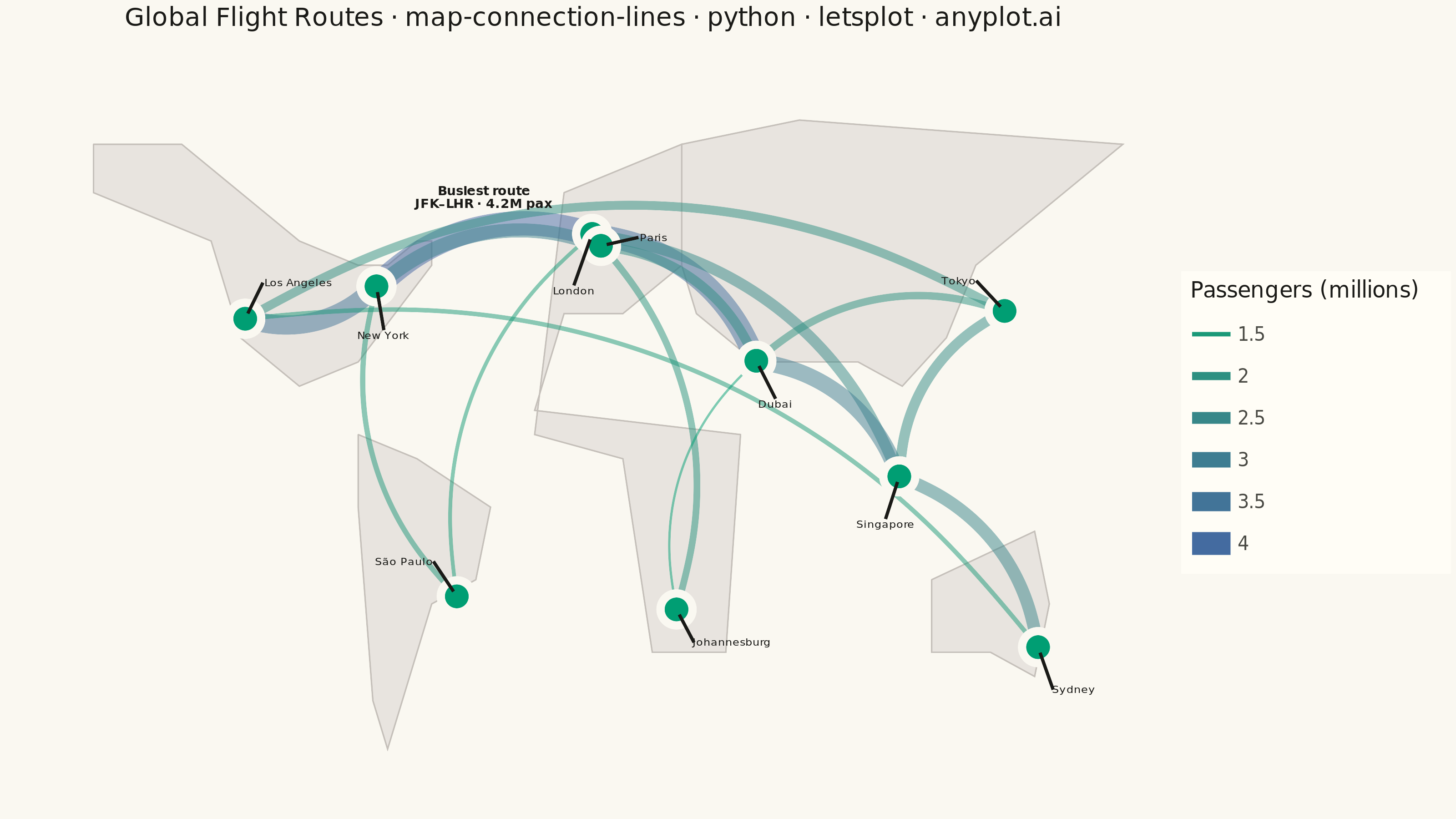
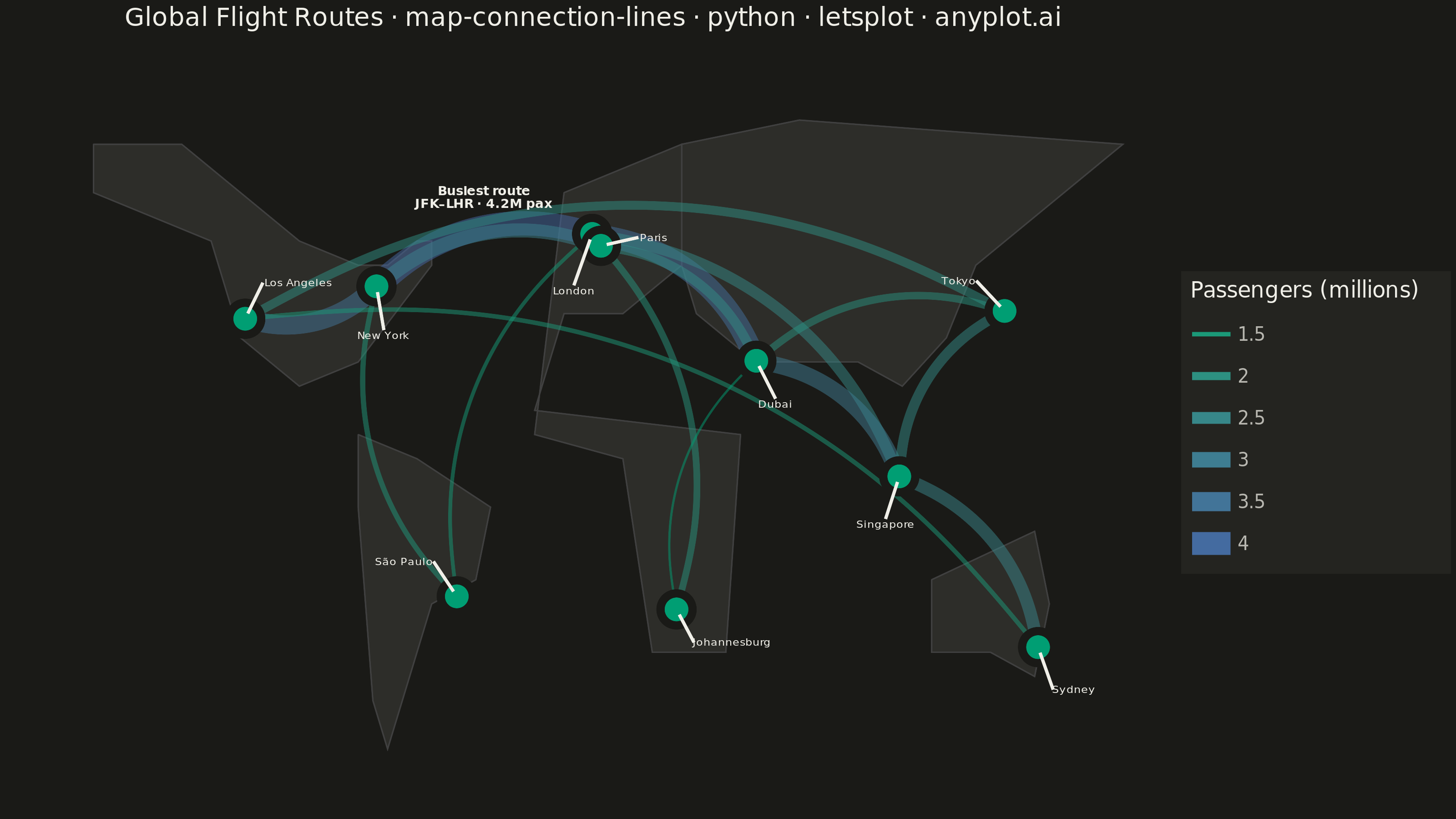
A geographic map visualization showing connection lines (arcs or great circles) between pairs of locations. This plot excels at revealing spatial patterns in flows, routes, and relationships between places. The curved lines naturally represent shortest paths on Earth's surface while avoiding visual overlap with straight lines. Line properties like thickness or color can encode additional variables such as traffic volume or connection type.
""" anyplot.ai
map-connection-lines: Connection Lines Map (Origin-Destination)
Library: letsplot 4.10.1 | Python 3.13.13
Quality: 84/100 | Updated: 2026-05-28
"""

import os

import numpy as np
import pandas as pd
from lets_plot import (
    LetsPlot,
    aes,
    element_rect,
    element_text,
    geom_curve,
    geom_point,
    geom_polygon,
    geom_text,
    geom_text_repel,
    ggplot,
    ggsave,
    ggsize,
    guide_legend,
    labs,
    scale_color_gradient,
    scale_size,
    theme,
    theme_void,
    xlim,
    ylim,
)


LetsPlot.setup_html()

# Theme tokens
THEME = os.getenv("ANYPLOT_THEME", "light")
PAGE_BG = "#FAF8F1" if THEME == "light" else "#1A1A17"
ELEVATED_BG = "#FFFDF6" if THEME == "light" else "#242420"
INK = "#1A1A17" if THEME == "light" else "#F0EFE8"
INK_SOFT = "#4A4A44" if THEME == "light" else "#B8B7B0"
LAND_FILL = "#E8E4DF" if THEME == "light" else "#2D2D29"
LAND_BORDER = "#C5C0BA" if THEME == "light" else "#404040"

# Data: Major flight routes between world cities
np.random.seed(42)

airports = {
    "JFK": (-73.78, 40.64, "New York"),
    "LAX": (-118.41, 33.94, "Los Angeles"),
    "LHR": (-0.45, 51.47, "London"),
    "CDG": (2.55, 49.01, "Paris"),
    "DXB": (55.37, 25.25, "Dubai"),
    "HND": (139.78, 35.55, "Tokyo"),
    "SIN": (103.99, 1.36, "Singapore"),
    "SYD": (151.18, -33.94, "Sydney"),
    "GRU": (-46.47, -23.44, "São Paulo"),
    "JNB": (28.24, -26.14, "Johannesburg"),
}

routes = [
    ("JFK", "LHR", 4.2),
    ("JFK", "CDG", 2.8),
    ("JFK", "LAX", 3.5),
    ("LAX", "HND", 2.1),
    ("LAX", "SYD", 1.5),
    ("LHR", "DXB", 3.8),
    ("LHR", "SIN", 2.4),
    ("LHR", "JNB", 1.8),
    ("CDG", "DXB", 2.2),
    ("DXB", "SIN", 3.1),
    ("DXB", "HND", 1.9),
    ("SIN", "SYD", 2.6),
    ("SIN", "HND", 2.3),
    ("GRU", "LHR", 1.4),
    ("GRU", "JFK", 1.6),
    ("JNB", "DXB", 1.2),
]

route_data = []
for origin, dest, passengers in routes:
    o_lon, o_lat, _ = airports[origin]
    d_lon, d_lat, _ = airports[dest]
    route_data.append(
        {"origin_lon": o_lon, "origin_lat": o_lat, "dest_lon": d_lon, "dest_lat": d_lat, "passengers": passengers}
    )
df_routes = pd.DataFrame(route_data)

airport_data = [{"name": name, "lon": lon, "lat": lat} for _, (lon, lat, name) in airports.items()]
df_airports = pd.DataFrame(airport_data)

# Annotation: highlight busiest route JFK-LHR (4.2M passengers)
jfk_lon, jfk_lat, _ = airports["JFK"]
lhr_lon, lhr_lat, _ = airports["LHR"]
df_callout = pd.DataFrame(
    [{"x": (jfk_lon + lhr_lon) / 2, "y": (jfk_lat + lhr_lat) / 2 + 13, "label": "Busiest route\nJFK–LHR · 4.2M pax"}]
)

# Simplified world coastline polygons
world_coords = [
    # North America
    (-170, 70),
    (-140, 70),
    (-120, 60),
    (-100, 50),
    (-80, 45),
    (-70, 45),
    (-60, 50),
    (-55, 50),
    (-55, 45),
    (-80, 25),
    (-100, 20),
    (-120, 30),
    (-130, 50),
    (-170, 60),
    (-170, 70),
    (None, None),
    # South America
    (-80, 10),
    (-60, 5),
    (-35, -5),
    (-40, -20),
    (-55, -25),
    (-70, -55),
    (-75, -45),
    (-80, -5),
    (-80, 10),
    (None, None),
    # Europe/Africa
    (-10, 60),
    (30, 70),
    (40, 65),
    (30, 45),
    (10, 35),
    (-10, 35),
    (-20, 15),
    (50, 10),
    (45, -35),
    (20, -35),
    (10, 5),
    (-20, 10),
    (-10, 60),
    (None, None),
    # Asia
    (30, 70),
    (70, 75),
    (180, 70),
    (160, 60),
    (140, 50),
    (130, 45),
    (120, 30),
    (105, 20),
    (90, 25),
    (70, 25),
    (55, 25),
    (45, 30),
    (35, 35),
    (30, 45),
    (30, 70),
    (None, None),
    # Australia
    (115, -20),
    (150, -10),
    (155, -25),
    (150, -40),
    (135, -35),
    (115, -35),
    (115, -20),
]

polygons = []
current_poly = []
for lon, lat in world_coords:
    if lon is None:
        if current_poly:
            polygons.append(current_poly)
            current_poly = []
    else:
        current_poly.append((lon, lat))
if current_poly:
    polygons.append(current_poly)

world_data = []
for i, poly in enumerate(polygons):
    for lon, lat in poly:
        world_data.append({"x": lon, "y": lat, "group": i})
df_world = pd.DataFrame(world_data)

# Title font size scaled to length
title = "Global Flight Routes · map-connection-lines · python · letsplot · anyplot.ai"
n = len(title)
ratio = 67 / n if n > 67 else 1.0
title_fontsize = max(11, round(16 * ratio))

# Plot
plot = (
    ggplot()
    + geom_polygon(data=df_world, mapping=aes(x="x", y="y", group="group"), fill=LAND_FILL, color=LAND_BORDER, size=0.3)
    + geom_curve(
        data=df_routes,
        mapping=aes(
            x="origin_lon", y="origin_lat", xend="dest_lon", yend="dest_lat", size="passengers", color="passengers"
        ),
        curvature=-0.3,
        alpha=0.5,
    )
    + geom_point(
        data=df_airports, mapping=aes(x="lon", y="lat"), size=6, color=PAGE_BG, fill="#009E73", shape=21, stroke=2
    )
    + geom_text_repel(
        data=df_airports,
        mapping=aes(x="lon", y="lat", label="name"),
        size=3,
        color=INK,
        seed=42,
        point_padding=5,
        box_padding=3,
        max_overlaps=20,
    )
    + geom_text(
        data=df_callout, mapping=aes(x="x", y="y", label="label"), size=3.5, color=INK, hjust=0.5, fontface="bold"
    )
    + scale_size(range=[0.5, 6], name="Passengers (millions)", guide=guide_legend())
    + scale_color_gradient(low="#009E73", high="#4467A3", name="Passengers (millions)", guide=guide_legend())
    + labs(title=title)
    + theme_void()
    + theme(
        plot_background=element_rect(fill=PAGE_BG, color=PAGE_BG),
        plot_title=element_text(size=title_fontsize, hjust=0.5, color=INK),
        legend_title=element_text(size=12, color=INK),
        legend_text=element_text(size=10, color=INK_SOFT),
        legend_position="right",
        legend_background=element_rect(fill=ELEVATED_BG, color=INK_SOFT),
    )
    + ggsize(800, 450)
    + xlim(-180, 180)
    + ylim(-60, 85)
)

ggsave(plot, f"plot-{THEME}.png", path=".", scale=4)
ggsave(plot, f"plot-{THEME}.html", path=".")
Runnable source as JSON, for any HTTP client: https://api.anyplot.ai/specs/map-connection-lines/letsplot/code. Any spec id and library id listed in llms-full.txt fit the same URL shape; every URL below is complete and callable.
{
  "spec_id": "map-connection-lines",
  "language": "python",
  "library": "letsplot",
  "page": "https://anyplot.ai/map-connection-lines/python/letsplot",
  "hub": "https://anyplot.ai/map-connection-lines",
  "code_json": "https://api.anyplot.ai/specs/map-connection-lines/letsplot/code",
  "spec_json": "https://api.anyplot.ai/specs/map-connection-lines",
  "render_light_png": "https://storage.googleapis.com/anyplot-images/plots/map-connection-lines/python/letsplot/plot-light.png",
  "render_dark_png": "https://storage.googleapis.com/anyplot-images/plots/map-connection-lines/python/letsplot/plot-dark.png",
  "interactive_light_html": "https://storage.googleapis.com/anyplot-images/plots/map-connection-lines/python/letsplot/plot-light.html",
  "interactive_dark_html": "https://storage.googleapis.com/anyplot-images/plots/map-connection-lines/python/letsplot/plot-dark.html",
  "quality_score": 84.0,
  "license": "MIT",
  "guide": "https://anyplot.ai/llms.txt"
}
Part of Connection Lines Map (Origin-Destination) on anyplot.ai.