The same plot in 14 other libraries — Python: Altair, Bokeh, lets-plot, Matplotlib, Plotly, plotnine, Pygal, Seaborn; R: ggplot2; JavaScript: Chart.js, D3.js, Apache ECharts, Highcharts, MUI X Charts. Compare all 15 side by side: Connection Lines Map (Origin-Destination) in Python, R, Julia and JavaScript.
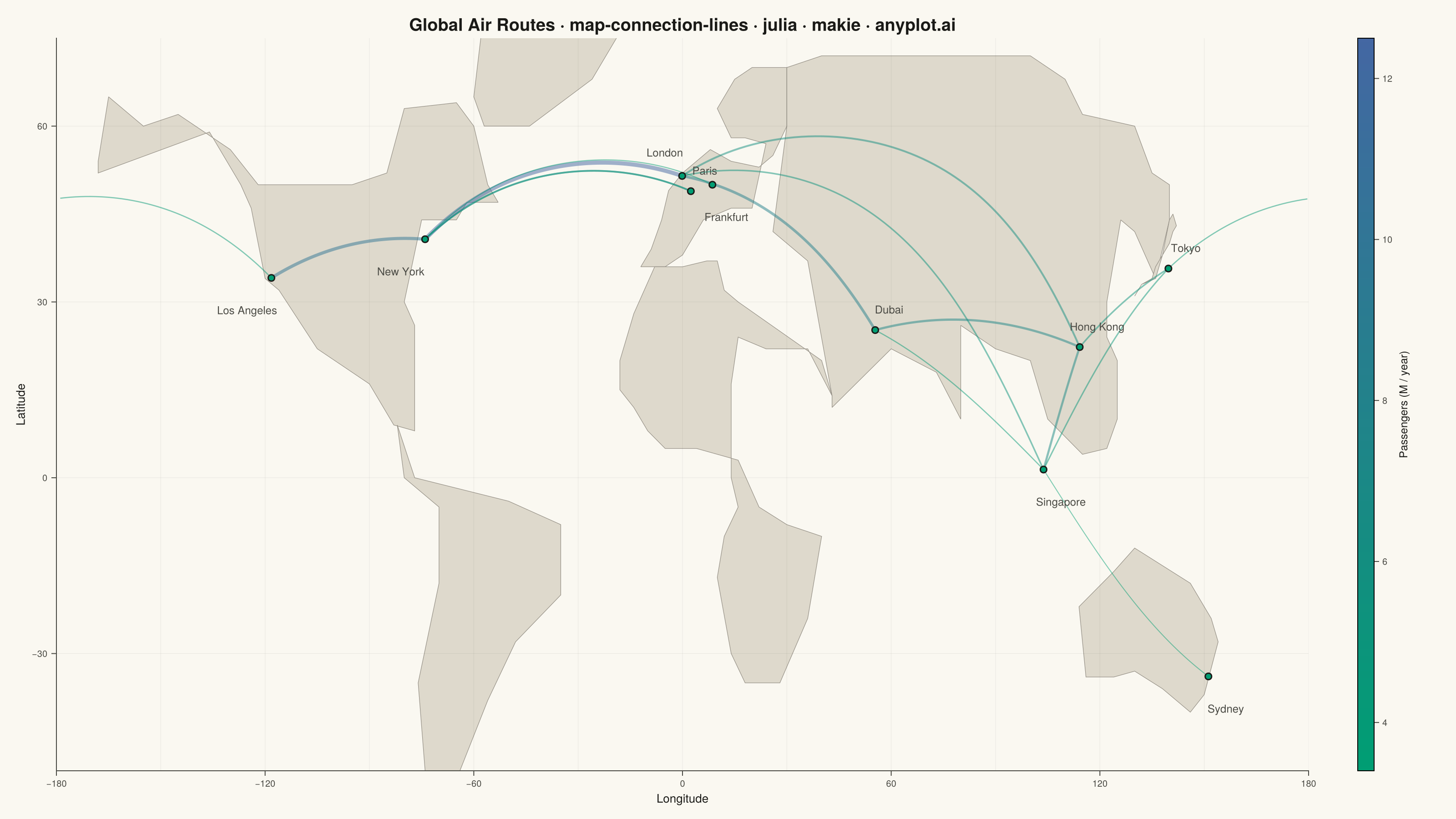
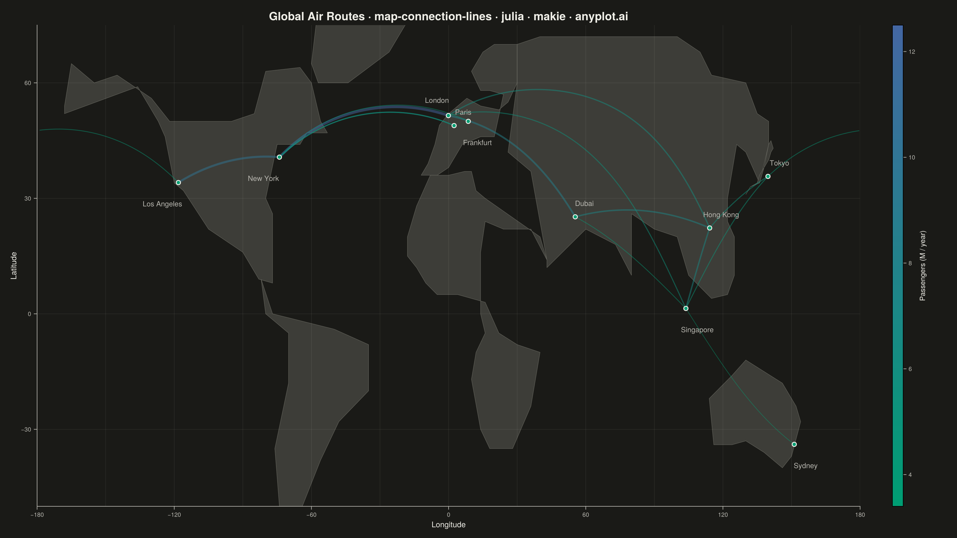
A geographic map visualization showing connection lines (arcs or great circles) between pairs of locations. This plot excels at revealing spatial patterns in flows, routes, and relationships between places. The curved lines naturally represent shortest paths on Earth's surface while avoiding visual overlap with straight lines. Line properties like thickness or color can encode additional variables such as traffic volume or connection type.
# anyplot.ai
# map-connection-lines: Connection Lines Map (Origin-Destination)
# Library: makie 0.22.10 | Julia 1.11.9
# Quality: 88/100 | Created: 2026-05-28

using CairoMakie
using Colors
using Random

Random.seed!(42)

# Theme tokens
const THEME       = get(ENV, "ANYPLOT_THEME", "light")
const PAGE_BG     = THEME == "light" ? colorant"#FAF8F1" : colorant"#1A1A17"
const INK         = THEME == "light" ? colorant"#1A1A17" : colorant"#F0EFE8"
const INK_SOFT    = THEME == "light" ? colorant"#4A4A44" : colorant"#B8B7B0"
const INK_MUTED   = THEME == "light" ? colorant"#6B6A63" : colorant"#A8A79F"

# Land and coastline colors (theme-adaptive)
const LAND_FILL   = THEME == "light" ?
    RGBAf(0.87f0, 0.85f0, 0.80f0, 1.0f0) :
    RGBAf(0.24f0, 0.24f0, 0.22f0, 1.0f0)
const COAST_COLOR = THEME == "light" ?
    RGBAf(0.58f0, 0.56f0, 0.52f0, 1.0f0) :
    RGBAf(0.40f0, 0.40f0, 0.37f0, 1.0f0)

const GRAT_ALPHA  = THEME == "light" ? 0.08f0 : 0.13f0
const GRAT_COLOR  = THEME == "light" ?
    RGBAf(26f0/255f0, 26f0/255f0, 23f0/255f0, GRAT_ALPHA) :
    RGBAf(240f0/255f0, 239f0/255f0, 232f0/255f0, GRAT_ALPHA)

# Sequential colormap: anyplot brand green → blue (single-polarity continuous)
const ANYPLOT_SEQ = cgrad([colorant"#009E73", colorant"#4467A3"])
const SEQ_R1, SEQ_G1, SEQ_B1 = 0f0/255f0,  158f0/255f0, 115f0/255f0   # #009E73
const SEQ_R2, SEQ_G2, SEQ_B2 = 68f0/255f0, 103f0/255f0, 163f0/255f0   # #4467A3

# Airport data: (name, lat, lon)
const airport_names = [
    "London", "New York", "Dubai", "Singapore",
    "Tokyo", "Sydney", "Paris", "Los Angeles",
    "Hong Kong", "Frankfurt",
]
const airport_lats = Float64[
     51.5,  40.7,  25.2,   1.4,
     35.7, -33.9,  48.9,  34.1,
     22.3,  50.0,
]
const airport_lons = Float64[
     -0.1, -74.0,  55.4, 103.8,
    139.7, 151.2,   2.4, -118.2,
    114.2,   8.6,
]

# Connections: (origin_idx, dest_idx, annual_passengers_millions)
const connections = [
    (1, 2, 12.5), (1, 3,  8.3), (1, 9,  6.1), (1, 4,  5.2),
    (2, 8,  9.8), (2, 7,  5.7), (3, 9,  7.2), (3, 4,  4.1),
    (9, 4,  6.8), (4, 5,  4.8), (4, 6,  3.4), (5, 9,  5.3),
    (5, 8,  4.2), (7, 2,  5.7), (10, 2, 3.9),
]

const volumes = Float64[c[3] for c in connections]
const vmin = minimum(volumes)
const vmax = maximum(volumes)

# Simplified continent polygon data as (lon, lat) tuple vectors.
# These are approximate shapes for geographic context; internal seas may appear as land.
# poly! auto-closes each polygon (last point connects back to first).
const _CONTINENTS_RAW = [
    # North America (clockwise from NW Alaska)
    [(-165,65),(-168,54),(-168,52),(-136,59),(-127,50),(-124,46),
     (-120,34),(-116,32),(-105,22),(-90,16),(-83,9),(-77,8),
     (-77,26),(-80,30),(-75,44),(-70,44),(-65,44),(-62,47),
     (-55,47),(-53,47),(-56,50),(-60,60),(-65,64),(-80,63),
     (-85,52),(-95,50),(-110,50),(-122,50),(-130,56),(-145,62),(-155,60)],
    # South America
    [(-82,9),(-77,0),(-50,-4),(-35,-8),(-35,-20),(-48,-28),
     (-56,-38),(-68,-56),(-74,-50),(-76,-35),(-70,-18),(-70,-5),(-80,0)],
    # Europe (Med coast → Atlantic → N Europe → back via Baltic states and Med)
    [(-12,36),(-9,39),(-6,44),(-4,49),(0,52),(8,56),(14,54),
     (22,53),(26,55),(30,60),(30,70),(20,70),(15,68),(10,63),
     (14,58),(18,58),(24,57),(20,46),(14,46),(6,44),(0,38),(-5,36)],
    # Asia: Turkey/Bosphorus → Middle East → India → SE Asia → China → Russia Arctic
    [(26,42),(36,37),(43,14),(43,12),(60,22),(73,18),(80,10),
     (80,26),(90,22),(100,20),(105,10),(115,4),(122,5),(125,10),
     (125,20),(122,24),(122,30),(126,44),(130,42),(136,34),
     (140,44),(140,50),(135,52),(130,60),(115,62),(110,68),
     (100,72),(80,72),(60,72),(40,72),(30,70),(30,60)],
    # Africa
    [(-18,15),(-14,12),(-10,8),(-5,5),(4,5),(10,4),(16,3),
     (22,-5),(30,-8),(40,-10),(36,-24),(28,-35),(18,-35),
     (14,-30),(10,-17),(12,-10),(16,-5),(14,0),(14,8),(14,16),
     (16,24),(24,22),(36,22),(43,14),(40,20),(16,30),(12,32),
     (10,37),(7,37),(0,36),(-5,36),(-8,36),(-14,28),(-18,20)],
    # Australia
    [(114,-22),(116,-34),(124,-34),(130,-33),(138,-36),(146,-40),
     (150,-37),(154,-28),(152,-24),(146,-18),(138,-15),(130,-12),(124,-16)],
    # Japan (Honshu main island, simplified)
    [(130,31),(132,33),(135,34),(136,36),(138,38),(140,40),
     (141,42),(142,43),(141,45),(140,44),(138,38),(136,34),(132,33)],
    # Greenland (partially visible above latitude crop)
    [(-44,83),(-18,77),(-18,76),(-26,68),(-44,60),(-57,60),(-60,65),(-58,75)],
]
const CONTINENTS = [[Point2f(p[1], p[2]) for p in c] for c in _CONTINENTS_RAW]

# Figure: landscape 1600×900 → 3200×1800 at px_per_unit=2
const title_str = "Global Air Routes · map-connection-lines · julia · makie · anyplot.ai"
const title_sz  = round(Int, 20 * min(1.0, 67 / length(title_str)))

fig = Figure(
    size            = (1600, 900),
    fontsize        = 12,
    backgroundcolor = PAGE_BG,
)

ax = Axis(
    fig[1, 1];
    title               = title_str,
    titlesize           = title_sz,
    titlecolor          = INK,
    xlabel              = "Longitude",
    ylabel              = "Latitude",
    xlabelsize          = 13,
    ylabelsize          = 13,
    xlabelcolor         = INK,
    ylabelcolor         = INK,
    xticklabelsize      = 10,
    yticklabelsize      = 10,
    xticklabelcolor     = INK_SOFT,
    yticklabelcolor     = INK_SOFT,
    xtickcolor          = INK_SOFT,
    ytickcolor          = INK_SOFT,
    backgroundcolor     = PAGE_BG,
    topspinevisible     = false,
    rightspinevisible   = false,
    leftspinecolor      = INK_SOFT,
    bottomspinecolor    = INK_SOFT,
    xgridvisible        = false,
    ygridvisible        = false,
    limits              = (-180, 180, -50, 75),
    xticks              = -180:60:180,
    yticks              = [-30, 0, 30, 60],
)

# Base map: simplified continent fills (drawn first, behind all other elements)
for pts in CONTINENTS
    poly!(ax, pts; color = LAND_FILL, strokecolor = COAST_COLOR, strokewidth = 0.6)
end

# Graticule: reference grid lines for geographic context
for lon in -180:30:180
    lines!(ax, [Float64(lon), Float64(lon)], [-50.0, 75.0];
        color = GRAT_COLOR, linewidth = 0.5)
end
for lat in -30:30:60
    lines!(ax, [-180.0, 180.0], [Float64(lat), Float64(lat)];
        color = GRAT_COLOR, linewidth = 0.5)
end

# Connection arcs: great-circle paths via SLERP, colored by passenger volume
for (oi, di, volume) in connections
    φ1 = deg2rad(airport_lats[oi]);  λ1 = deg2rad(airport_lons[oi])
    φ2 = deg2rad(airport_lats[di]);  λ2 = deg2rad(airport_lons[di])
    d_ang = acos(clamp(sin(φ1) * sin(φ2) + cos(φ1) * cos(φ2) * cos(λ2 - λ1), -1.0, 1.0))

    arc_lons = Float64[]
    arc_lats = Float64[]
    n_pts = 80
    for i in 0:n_pts
        t = i / n_pts
        A = sin((1 - t) * d_ang) / sin(d_ang)
        B = sin(t * d_ang) / sin(d_ang)
        x = A * cos(φ1) * cos(λ1) + B * cos(φ2) * cos(λ2)
        y = A * cos(φ1) * sin(λ1) + B * cos(φ2) * sin(λ2)
        z = A * sin(φ1) + B * sin(φ2)
        lon_pt = rad2deg(atan(y, x))
        lat_pt = rad2deg(atan(z, sqrt(x^2 + y^2)))
        if !isempty(arc_lons) && abs(lon_pt - arc_lons[end]) > 180
            push!(arc_lons, NaN)
            push!(arc_lats, NaN)
        end
        push!(arc_lons, lon_pt)
        push!(arc_lats, lat_pt)
    end

    nv = Float32((volume - vmin) / (vmax - vmin))
    arc_color = RGBAf(
        SEQ_R1 + (SEQ_R2 - SEQ_R1) * nv,
        SEQ_G1 + (SEQ_G2 - SEQ_G1) * nv,
        SEQ_B1 + (SEQ_B2 - SEQ_B1) * nv,
        0.50f0,   # within spec's recommended 0.3–0.6
    )
    lines!(ax, arc_lons, arc_lats;
        color     = arc_color,
        linewidth = 1.0 + 3.5 * nv,
    )
end

# Airport endpoint markers
scatter!(ax, airport_lons, airport_lats;
    color       = colorant"#009E73",
    markersize  = 10,
    strokewidth = 1.5,
    strokecolor = INK,
)

# Airport labels with manual offsets to minimise overlap in dense clusters
const label_offsets = [
    (-5.0,  4.0),   # London
    (-7.0, -5.5),   # New York
    ( 4.0,  3.5),   # Dubai
    ( 5.0, -5.5),   # Singapore
    ( 5.0,  3.5),   # Tokyo
    ( 5.0, -5.5),   # Sydney
    ( 4.0,  3.5),   # Paris
    (-7.0, -5.5),   # Los Angeles
    ( 5.0,  3.5),   # Hong Kong
    ( 4.0, -5.5),   # Frankfurt
]

for (i, name) in enumerate(airport_names)
    dx, dy = label_offsets[i]
    text!(ax, airport_lons[i] + dx, airport_lats[i] + dy;
        text     = name,
        fontsize = 12,
        color    = INK_SOFT,
        align    = (:center, :center),
    )
end

# Colorbar: maps passenger volume (M/year) to the sequential palette
Colorbar(fig[1, 2];
    colormap       = ANYPLOT_SEQ,
    limits         = (vmin, vmax),
    label          = "Passengers (M / year)",
    labelsize      = 12,
    labelcolor     = INK,
    ticklabelsize  = 10,
    ticklabelcolor = INK_SOFT,
    tickcolor      = INK_SOFT,
    width          = 18,
    tellheight     = false,
)

colsize!(fig.layout, 2, Fixed(90))

save("plot-$(THEME).png", fig; px_per_unit = 2)
Runnable source as JSON, for any HTTP client: https://api.anyplot.ai/specs/map-connection-lines/makie/code. Any spec id and library id listed in llms-full.txt fit the same URL shape; every URL below is complete and callable.
{
  "spec_id": "map-connection-lines",
  "language": "julia",
  "library": "makie",
  "page": "https://anyplot.ai/map-connection-lines/julia/makie",
  "hub": "https://anyplot.ai/map-connection-lines",
  "code_json": "https://api.anyplot.ai/specs/map-connection-lines/makie/code",
  "spec_json": "https://api.anyplot.ai/specs/map-connection-lines",
  "render_light_png": "https://storage.googleapis.com/anyplot-images/plots/map-connection-lines/julia/makie/plot-light.png",
  "render_dark_png": "https://storage.googleapis.com/anyplot-images/plots/map-connection-lines/julia/makie/plot-dark.png",
  "quality_score": 88.0,
  "license": "MIT",
  "guide": "https://anyplot.ai/llms.txt"
}
Part of Connection Lines Map (Origin-Destination) on anyplot.ai.