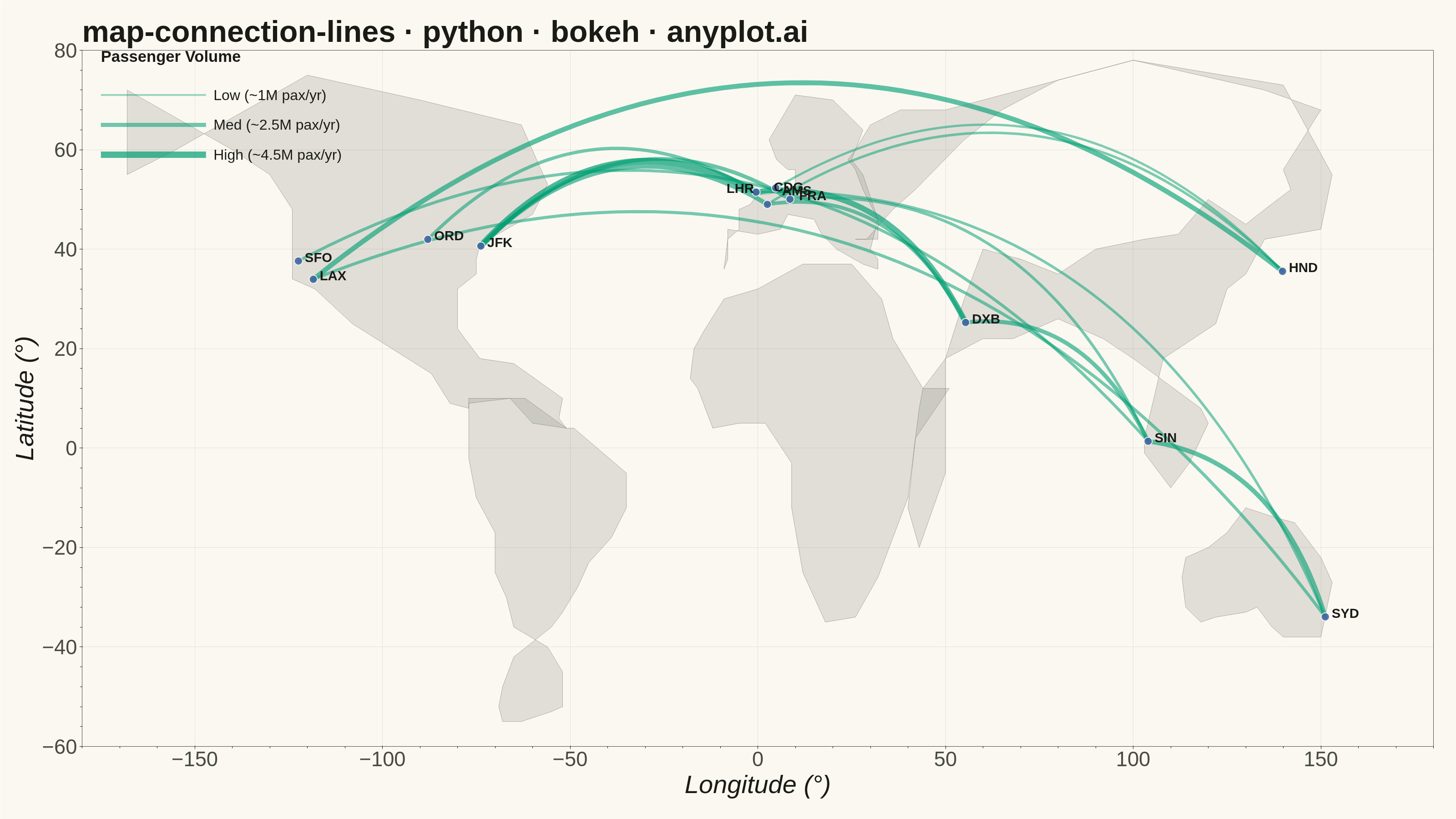
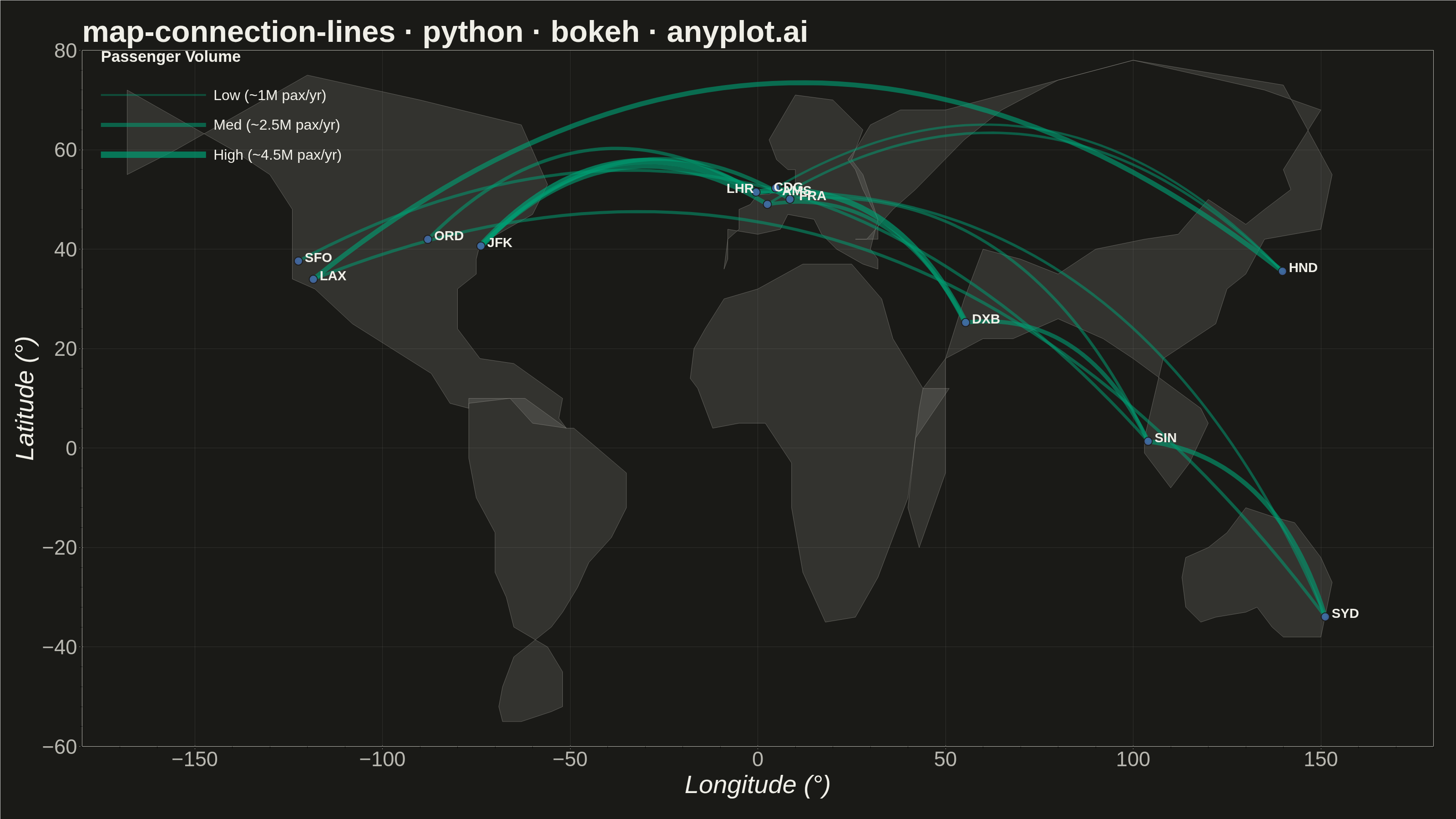
A geographic map visualization showing connection lines (arcs or great circles) between pairs of locations. This plot excels at revealing spatial patterns in flows, routes, and relationships between places. The curved lines naturally represent shortest paths on Earth's surface while avoiding visual overlap with straight lines. Line properties like thickness or color can encode additional variables such as traffic volume or connection type.
""" anyplot.ai
map-connection-lines: Connection Lines Map (Origin-Destination)
Library: bokeh 3.9.0 | Python 3.13.13
Quality: 86/100 | Updated: 2026-05-28
"""

import os
import time
from pathlib import Path

import numpy as np
from bokeh.io import output_file, save
from bokeh.models import ColumnDataSource, HoverTool
from bokeh.plotting import figure
from selenium import webdriver
from selenium.webdriver.chrome.options import Options


# Theme tokens
THEME = os.getenv("ANYPLOT_THEME", "light")
PAGE_BG = "#FAF8F1" if THEME == "light" else "#1A1A17"
ELEVATED_BG = "#FFFDF6" if THEME == "light" else "#242420"
INK = "#1A1A17" if THEME == "light" else "#F0EFE8"
INK_SOFT = "#4A4A44" if THEME == "light" else "#B8B7B0"
INK_MUTED = "#6B6A63" if THEME == "light" else "#A8A79F"

IMPRINT_PALETTE = ["#009E73", "#C475FD", "#4467A3", "#BD8233", "#AE3030", "#2ABCCD", "#954477", "#99B314"]
BRAND = IMPRINT_PALETTE[0]  # green — connection lines (first series)
ACCENT = IMPRINT_PALETTE[2]  # blue — airport markers

# Simplified continent outlines (approximate polygons for geographic context)
CONT_LON = [
    # Africa
    [-18, -17, -14, -9, 0, 12, 25, 33, 36, 44, 51, 42, 40, 36, 32, 26, 18, 12, 9, 9, 2, -5, -12, -16, -18],
    # Europe
    [
        -9,
        -8,
        -8,
        0,
        6,
        8,
        15,
        17,
        21,
        28,
        32,
        32,
        30,
        32,
        28,
        25,
        28,
        20,
        10,
        3,
        5,
        8,
        10,
        10,
        10,
        5,
        3,
        0,
        -2,
        -5,
        -5,
        -8,
        -9,
    ],
    # North America
    [
        -168,
        -140,
        -130,
        -124,
        -124,
        -118,
        -108,
        -87,
        -82,
        -77,
        -77,
        -66,
        -60,
        -51,
        -53,
        -52,
        -65,
        -74,
        -80,
        -80,
        -75,
        -75,
        -74,
        -67,
        -60,
        -56,
        -63,
        -90,
        -120,
        -155,
        -168,
        -168,
    ],
    # South America
    [
        -77,
        -62,
        -51,
        -49,
        -35,
        -35,
        -39,
        -45,
        -48,
        -52,
        -55,
        -65,
        -68,
        -69,
        -68,
        -63,
        -55,
        -52,
        -52,
        -56,
        -65,
        -67,
        -70,
        -70,
        -75,
        -77,
        -77,
    ],
    # Asia (simplified)
    [
        26,
        29,
        36,
        42,
        55,
        65,
        80,
        100,
        140,
        153,
        150,
        135,
        130,
        125,
        122,
        108,
        103,
        103,
        110,
        115,
        120,
        118,
        100,
        92,
        80,
        68,
        60,
        50,
        44,
        43,
        42,
        40,
        43,
        50,
        50,
        50,
        55,
        60,
        70,
        80,
        90,
        103,
        112,
        120,
        130,
        135,
        142,
        140,
        145,
        150,
        135,
        100,
        60,
        50,
        38,
        30,
        26,
        24,
        26,
        28,
        32,
        32,
        26,
    ],
    # Australia
    [114, 113, 114, 118, 122, 130, 133, 137, 140, 150, 153, 150, 143, 138, 130, 125, 120, 114],
]
CONT_LAT = [
    # Africa
    [14, 20, 24, 30, 32, 37, 37, 30, 22, 12, 12, 2, -10, -18, -26, -34, -35, -25, -12, -3, 5, 5, 4, 12, 14],
    # Europe
    [
        36,
        38,
        44,
        43,
        44,
        47,
        46,
        43,
        40,
        37,
        36,
        38,
        40,
        46,
        55,
        58,
        64,
        70,
        71,
        62,
        58,
        56,
        56,
        55,
        52,
        52,
        51,
        51,
        49,
        48,
        44,
        42,
        36,
    ],
    # North America
    [
        72,
        60,
        55,
        48,
        34,
        32,
        25,
        15,
        9,
        8,
        9,
        10,
        5,
        4,
        6,
        10,
        17,
        18,
        24,
        32,
        35,
        38,
        41,
        44,
        47,
        53,
        65,
        70,
        75,
        60,
        55,
        72,
    ],
    # South America
    [
        10,
        10,
        4,
        4,
        -5,
        -12,
        -18,
        -23,
        -28,
        -33,
        -36,
        -42,
        -48,
        -52,
        -55,
        -55,
        -53,
        -52,
        -45,
        -40,
        -36,
        -30,
        -25,
        -17,
        -10,
        -2,
        10,
    ],
    # Asia
    [
        42,
        42,
        48,
        52,
        62,
        68,
        74,
        78,
        73,
        55,
        44,
        42,
        35,
        32,
        25,
        18,
        2,
        -1,
        -8,
        -3,
        5,
        8,
        18,
        22,
        26,
        22,
        22,
        18,
        12,
        8,
        2,
        -12,
        -20,
        -5,
        12,
        18,
        30,
        40,
        38,
        35,
        40,
        42,
        43,
        50,
        45,
        48,
        52,
        56,
        62,
        68,
        72,
        78,
        70,
        68,
        68,
        65,
        60,
        58,
        56,
        52,
        46,
        42,
        42,
    ],
    # Australia
    [-22, -26, -32, -35, -34, -33, -32, -36, -38, -38, -27, -22, -15, -14, -12, -17, -20, -22],
]

# Data: Major international flight routes between hub airports
airports = {
    "JFK": (40.6413, -73.7781),  # New York
    "LHR": (51.4700, -0.4543),  # London
    "CDG": (49.0097, 2.5479),  # Paris
    "DXB": (25.2532, 55.3657),  # Dubai
    "SIN": (1.3644, 103.9915),  # Singapore
    "HND": (35.5494, 139.7798),  # Tokyo
    "SYD": (-33.9399, 151.1753),  # Sydney
    "LAX": (33.9416, -118.4085),  # Los Angeles
    "SFO": (37.6213, -122.3790),  # San Francisco
    "ORD": (41.9742, -87.9073),  # Chicago
    "FRA": (50.0379, 8.5622),  # Frankfurt
    "AMS": (52.3105, 4.7683),  # Amsterdam
}

routes = [
    ("JFK", "LHR", 4.5),
    ("JFK", "CDG", 2.8),
    ("LAX", "HND", 3.2),
    ("SFO", "SIN", 1.5),
    ("LHR", "DXB", 3.8),
    ("CDG", "DXB", 2.1),
    ("DXB", "SIN", 2.5),
    ("SIN", "SYD", 2.9),
    ("LHR", "SYD", 1.2),
    ("JFK", "FRA", 2.3),
    ("ORD", "LHR", 1.8),
    ("LAX", "SYD", 1.6),
    ("FRA", "SIN", 1.4),
    ("AMS", "HND", 0.9),
    ("CDG", "HND", 1.1),
]

# Build curved arc data (parabolic perpendicular offset in lat/lon space)
line_xs, line_ys, line_widths, line_alphas = [], [], [], []
route_labels, passenger_volumes = [], []
volumes = [r[2] for r in routes]
min_vol, max_vol = min(volumes), max(volumes)

for origin, dest, volume in routes:
    o_lat, o_lon = airports[origin]
    d_lat, d_lon = airports[dest]
    t = np.linspace(0, 1, 60)
    arc_lons = o_lon + (d_lon - o_lon) * t
    arc_lats = o_lat + (d_lat - o_lat) * t
    dx, dy = d_lon - o_lon, d_lat - o_lat
    dist = np.sqrt(dx**2 + dy**2)
    mid_offset = dist * 0.15
    curve = 4 * t * (1 - t) * mid_offset
    if dist > 0:
        perp_x, perp_y = -dy / dist, dx / dist
    else:
        perp_x, perp_y = 0.0, 0.0
    arc_lons = arc_lons + perp_x * curve
    arc_lats = arc_lats + perp_y * curve
    line_xs.append(arc_lons.tolist())
    line_ys.append(arc_lats.tolist())
    normalized = (volume - min_vol) / (max_vol - min_vol) if max_vol > min_vol else 0.5
    line_widths.append(5 + normalized * 9)
    line_alphas.append(0.5 + normalized * 0.2)
    route_labels.append(f"{origin} → {dest}")
    passenger_volumes.append(f"{volume}M pax/year")

# Airport marker data
airport_names = list(airports.keys())
airport_lons = [airports[a][1] for a in airport_names]
airport_lats = [airports[a][0] for a in airport_names]

# Per-airport label offsets — push European cluster apart to prevent overlap
LABEL_OFFSETS = {
    "LHR": (-65, 8),  # west of dot; avoids CDG/AMS cluster to the right
    "AMS": (14, 22),  # above default; AMS is the northernmost hub
    "CDG": (14, -22),  # below default; CDG is the southernmost hub
    "FRA": (20, 8),  # slightly further right than default
}
airport_x_offsets = [LABEL_OFFSETS.get(a, (14, 8))[0] for a in airport_names]
airport_y_offsets = [LABEL_OFFSETS.get(a, (14, 8))[1] for a in airport_names]

# Data sources
line_source = ColumnDataSource(
    data={
        "xs": line_xs,
        "ys": line_ys,
        "line_width": line_widths,
        "alpha": line_alphas,
        "route": route_labels,
        "passengers": passenger_volumes,
    }
)
airport_source = ColumnDataSource(
    data={
        "x": airport_lons,
        "y": airport_lats,
        "name": airport_names,
        "x_off": airport_x_offsets,
        "y_off": airport_y_offsets,
    }
)
continent_source = ColumnDataSource(data={"xs": CONT_LON, "ys": CONT_LAT})

# Title font size (scales linearly if title exceeds 67-char baseline)
title = "map-connection-lines · python · bokeh · anyplot.ai"
n = len(title)
title_fs = f"{round(50 * (67 / n if n > 67 else 1.0))}pt"

# Figure — width/height are the exact PNG canvas dimensions
p = figure(
    width=3200,
    height=1800,
    title=title,
    x_range=(-180, 180),
    y_range=(-60, 80),
    x_axis_label="Longitude (°)",
    y_axis_label="Latitude (°)",
    toolbar_location=None,  # omit toolbar so PNG = exactly height=1800 px
    min_border_bottom=160,  # room for 34pt tick labels + 42pt x-axis label
    min_border_left=180,  # room for 34pt tick labels + 42pt y-axis label
    min_border_top=110,  # room for 50pt title
    min_border_right=50,
)

# Continent base map
p.patches(
    xs="xs",
    ys="ys",
    source=continent_source,
    fill_color=INK_MUTED,
    fill_alpha=0.18,
    line_color=INK_SOFT,
    line_width=0.8,
    line_alpha=0.5,
)

# Connection arcs — line width and alpha encode passenger volume
lines_renderer = p.multi_line(
    xs="xs",
    ys="ys",
    source=line_source,
    line_width="line_width",
    line_alpha="alpha",
    line_color=BRAND,
    line_cap="round",
)
p.add_tools(
    HoverTool(
        renderers=[lines_renderer], tooltips=[("Route", "@route"), ("Traffic", "@passengers")], line_policy="interp"
    )
)

# Airport markers
p.scatter(x="x", y="y", source=airport_source, size=18, color=ACCENT, line_color=PAGE_BG, line_width=2, alpha=0.9)
p.text(
    x="x",
    y="y",
    text="name",
    source=airport_source,
    x_offset="x_off",
    y_offset="y_off",
    text_font_size="22pt",
    text_color=INK,
    text_font_style="bold",
)

# Manual legend (upper-left Pacific — clear of all route clusters)
lx0, lx1 = -175, -147
ly_title, ly = 77, [71, 65, 59]
p.multi_line(xs=[[lx0, lx1]], ys=[[ly[0], ly[0]]], line_width=4, line_color=BRAND, line_alpha=0.4)
p.multi_line(xs=[[lx0, lx1]], ys=[[ly[1], ly[1]]], line_width=9, line_color=BRAND, line_alpha=0.55)
p.multi_line(xs=[[lx0, lx1]], ys=[[ly[2], ly[2]]], line_width=14, line_color=BRAND, line_alpha=0.7)
p.text(x=[lx1 + 2], y=[ly[0]], text=["Low (~1M pax/yr)"], text_font_size="24pt", text_color=INK, text_baseline="middle")
p.text(
    x=[lx1 + 2], y=[ly[1]], text=["Med (~2.5M pax/yr)"], text_font_size="24pt", text_color=INK, text_baseline="middle"
)
p.text(
    x=[lx1 + 2], y=[ly[2]], text=["High (~4.5M pax/yr)"], text_font_size="24pt", text_color=INK, text_baseline="middle"
)
p.text(x=[lx0], y=[ly_title], text=["Passenger Volume"], text_font_size="26pt", text_color=INK, text_font_style="bold")

# Theme-adaptive chrome
p.title.text_font_size = title_fs
p.title.text_color = INK
p.xaxis.axis_label_text_font_size = "42pt"
p.yaxis.axis_label_text_font_size = "42pt"
p.xaxis.major_label_text_font_size = "34pt"
p.yaxis.major_label_text_font_size = "34pt"
p.xaxis.axis_label_text_color = INK
p.yaxis.axis_label_text_color = INK
p.xaxis.major_label_text_color = INK_SOFT
p.yaxis.major_label_text_color = INK_SOFT
p.xaxis.axis_line_color = INK_SOFT
p.yaxis.axis_line_color = INK_SOFT
p.xaxis.major_tick_line_color = INK_SOFT
p.yaxis.major_tick_line_color = INK_SOFT
p.xgrid.grid_line_color = INK
p.ygrid.grid_line_color = INK
p.xgrid.grid_line_alpha = 0.1
p.ygrid.grid_line_alpha = 0.1
p.background_fill_color = PAGE_BG
p.border_fill_color = PAGE_BG
p.outline_line_color = INK_SOFT

# Save interactive HTML (required catalog artifact)
output_file(f"plot-{THEME}.html")
save(p)

# Screenshot with headless Chrome via Selenium
W, H = 3200, 1800
opts = Options()
for arg in (
    "--headless=new",
    "--no-sandbox",
    "--disable-dev-shm-usage",
    "--disable-gpu",
    f"--window-size={W},{H}",
    "--hide-scrollbars",
):
    opts.add_argument(arg)
driver = webdriver.Chrome(options=opts)
# Force exact viewport to W×H regardless of headless browser chrome overhead
driver.execute_cdp_cmd(
    "Emulation.setDeviceMetricsOverride", {"width": W, "height": H, "deviceScaleFactor": 1, "mobile": False}
)
driver.get(f"file://{Path(f'plot-{THEME}.html').resolve()}")
time.sleep(3)
driver.save_screenshot(f"plot-{THEME}.png")
driver.quit()
Runnable source as JSON, for any HTTP client: https://api.anyplot.ai/specs/map-connection-lines/bokeh/code. Any spec id and library id listed in llms-full.txt fit the same URL shape; every URL below is complete and callable.
{
  "spec_id": "map-connection-lines",
  "language": "python",
  "library": "bokeh",
  "page": "https://anyplot.ai/map-connection-lines/python/bokeh",
  "hub": "https://anyplot.ai/map-connection-lines",
  "code_json": "https://api.anyplot.ai/specs/map-connection-lines/bokeh/code",
  "spec_json": "https://api.anyplot.ai/specs/map-connection-lines",
  "render_light_png": "https://storage.googleapis.com/anyplot-images/plots/map-connection-lines/python/bokeh/plot-light.png",
  "render_dark_png": "https://storage.googleapis.com/anyplot-images/plots/map-connection-lines/python/bokeh/plot-dark.png",
  "interactive_light_html": "https://storage.googleapis.com/anyplot-images/plots/map-connection-lines/python/bokeh/plot-light.html",
  "interactive_dark_html": "https://storage.googleapis.com/anyplot-images/plots/map-connection-lines/python/bokeh/plot-dark.html",
  "quality_score": 86.0,
  "license": "MIT",
  "guide": "https://anyplot.ai/llms.txt"
}
Part of Connection Lines Map (Origin-Destination) on anyplot.ai.