The same plot in 12 other libraries — Python: Altair, Bokeh, lets-plot, Matplotlib, Plotly, plotnine, Pygal, Seaborn; R: ggplot2; JavaScript: Chart.js, D3.js, Apache ECharts. Compare all 13 side by side: Map with Tile Background in Python, R, Julia and JavaScript.
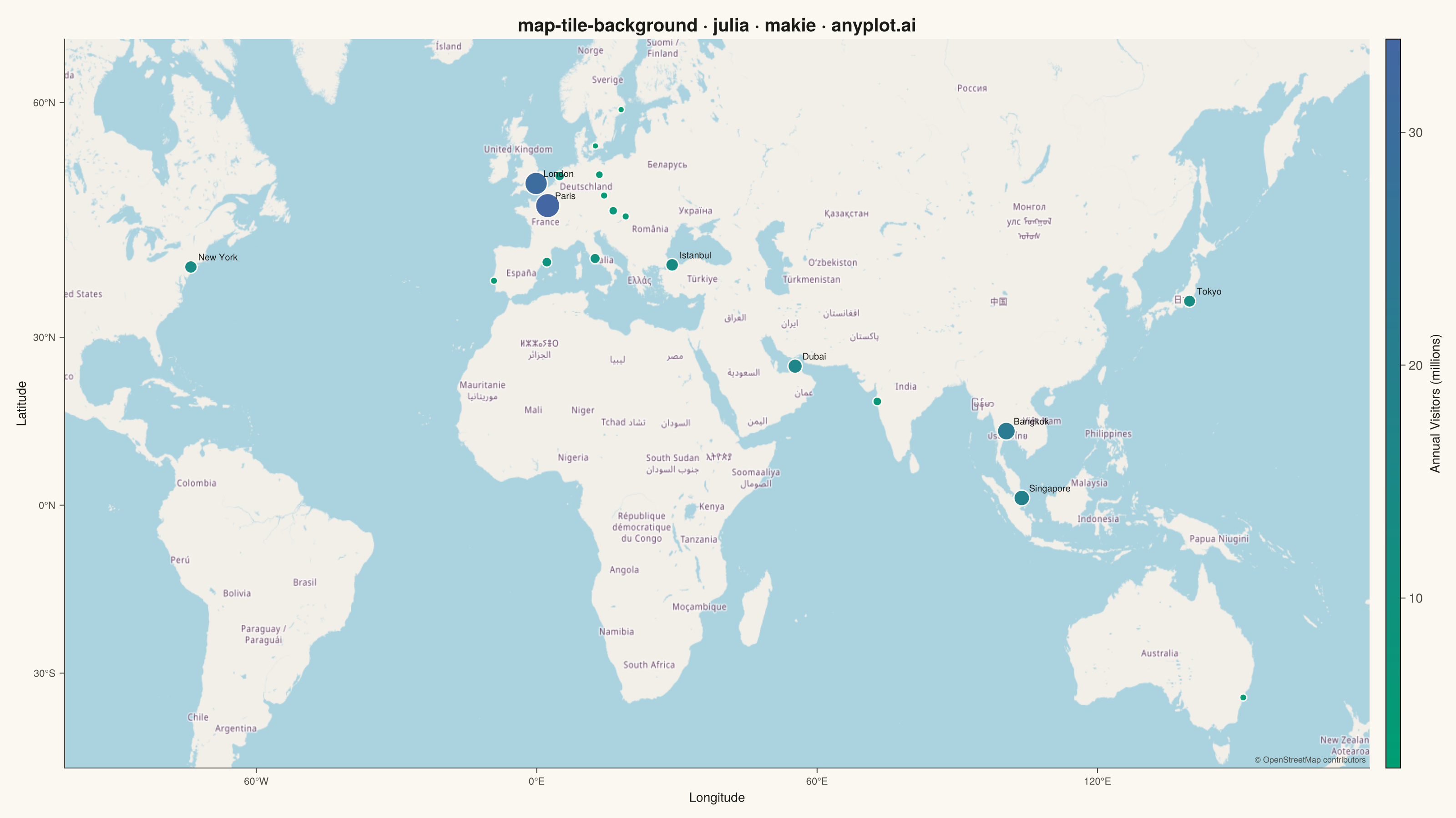
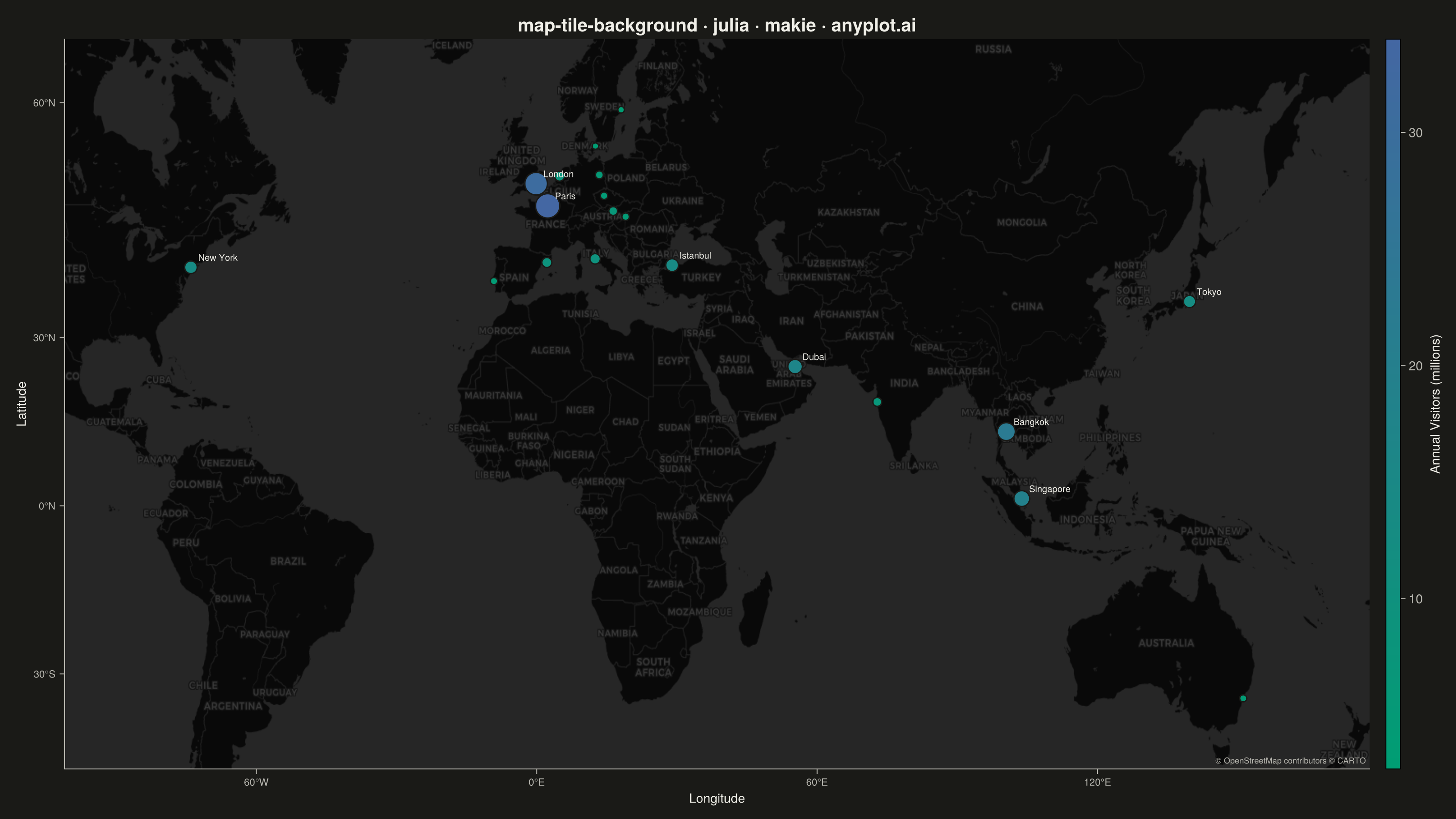
A map visualization that displays data points on top of tile-based backgrounds such as OpenStreetMap, Stamen, or satellite imagery. Unlike vector-based basemaps, tile backgrounds provide rich geographic context including street-level detail, terrain, or satellite imagery that loads dynamically as the user navigates. This visualization is essential for location-based analysis where real-world geographic context enhances data interpretation.
# anyplot.ai
# map-tile-background: Map with Tile Background
# Library: makie 0.22.10 | Julia 1.11.9
# Quality: 88/100 | Created: 2026-05-27

using CairoMakie
using Colors
using Random
using Downloads
using PNGFiles

Random.seed!(42)

# Theme tokens
const THEME       = get(ENV, "ANYPLOT_THEME", "light")
const PAGE_BG     = THEME == "light" ? colorant"#FAF8F1" : colorant"#1A1A17"
const INK         = THEME == "light" ? colorant"#1A1A17" : colorant"#F0EFE8"
const INK_SOFT    = THEME == "light" ? colorant"#4A4A44" : colorant"#B8B7B0"
const ANYPLOT_SEQ = cgrad([colorant"#009E73", colorant"#4467A3"])

# Theme-adaptive tile providers
const TILE_URL   = THEME == "light" ?
    "https://tile.openstreetmap.org/{z}/{x}/{y}.png" :
    "https://a.basemaps.cartocdn.com/dark_all/{z}/{x}/{y}.png"
const TILE_CREDIT = THEME == "light" ?
    "© OpenStreetMap contributors" :
    "© OpenStreetMap contributors © CARTO"

# Web Mercator helpers (EPSG:3857 slippy-map tile convention)
lat_to_merc(lat)     = log(tan(lat * π / 180) + 1 / cos(lat * π / 180))
merc_to_lat(m)       = atan(sinh(m)) * 180 / π
lon_to_tx(lon, z)    = clamp(floor(Int, (lon + 180) / 360 * (1 << z)), 0, (1 << z) - 1)
lat_to_ty(lat, z)    = clamp(floor(Int, (π - lat_to_merc(lat)) / (2π) * (1 << z)), 0, (1 << z) - 1)
tx_lon_west(tx, z)   = tx / (1 << z) * 360 - 180
tx_lon_east(tx, z)   = (tx + 1) / (1 << z) * 360 - 180
ty_merc_north(ty, z) = π * (1 - 2 * ty / (1 << z))
ty_merc_south(ty, z) = π * (1 - 2 * (ty + 1) / (1 << z))

# City data: major tourist destinations with annual visitor counts (millions)
const city_names = [
    "Paris", "London", "New York", "Tokyo", "Barcelona",
    "Rome", "Dubai", "Istanbul", "Amsterdam", "Singapore",
    "Sydney", "Bangkok", "Mumbai", "Berlin", "Prague",
    "Vienna", "Budapest", "Lisbon", "Copenhagen", "Stockholm",
]
const lons = Float64[
    2.35, -0.12, -74.0, 139.7, 2.17,
    12.5, 55.3, 28.98, 4.9, 103.8,
    151.2, 100.5, 72.88, 13.41, 14.42,
    16.37, 19.04, -9.14, 12.57, 18.07,
]
const lats = Float64[
    48.85, 51.51, 40.71, 35.68, 41.39,
    41.9, 25.2, 41.01, 52.37, 1.35,
    -33.87, 13.75, 19.08, 52.52, 50.08,
    48.21, 47.5, 38.72, 55.68, 59.33,
]
const visitors = Float64[
    34.0, 31.0, 13.6, 12.9, 9.0,
    9.7, 16.7, 14.0, 8.6, 19.1,
    3.8, 22.8, 7.0, 5.3, 4.4,
    6.8, 4.4, 4.1, 2.7, 2.9,
]

# Convert latitudes to Mercator Y for correct Web Mercator projection
y_merc       = lat_to_merc.(lats)
v_min        = minimum(visitors)
v_max        = maximum(visitors)
v_norm       = (visitors .- v_min) ./ (v_max - v_min)
marker_sizes = 10.0 .+ 28.0 .* v_norm

# Padded axis extent (12 % padding in each direction)
lon_pad      = (maximum(lons)   - minimum(lons))   * 0.12
merc_pad     = (maximum(y_merc) - minimum(y_merc)) * 0.12
ax_lon_min   = minimum(lons)   - lon_pad
ax_lon_max   = maximum(lons)   + lon_pad
ax_merc_min  = minimum(y_merc) - merc_pad
ax_merc_max  = maximum(y_merc) + merc_pad
pad_lat_north = merc_to_lat(ax_merc_max)
pad_lat_south = merc_to_lat(ax_merc_min)

# Tile grid parameters
const ZOOM    = 3
const TILE_PX = 256

tx_min = lon_to_tx(ax_lon_min, ZOOM)
tx_max = lon_to_tx(ax_lon_max, ZOOM)
ty_min = lat_to_ty(pad_lat_north, ZOOM)   # north edge → smaller tile y index
ty_max = lat_to_ty(pad_lat_south, ZOOM)   # south edge → larger tile y index

n_tx = tx_max - tx_min + 1
n_ty = ty_max - ty_min + 1

# Stitched raster: [pixel_x, pixel_y] where x = west→east, y = north→south
stitched = fill(RGBA{Float32}(0.87f0, 0.87f0, 0.87f0, 1.0f0), TILE_PX * n_tx, TILE_PX * n_ty)

mktempdir() do tmpdir
    for iy in 0:(n_ty - 1), ix in 0:(n_tx - 1)
        tx  = tx_min + ix
        ty  = ty_min + iy
        url = replace(TILE_URL,
            "{z}" => string(ZOOM), "{x}" => string(tx), "{y}" => string(ty))
        fpath = joinpath(tmpdir, "$(tx)_$(ty).png")
        try
            Downloads.download(url, fpath;
                headers = ["User-Agent" =>
                    "anyplot.ai static visualization; [email protected]"])
            tile_mat = PNGFiles.load(fpath)   # size = (height, width) = [row, col] = [y, x]
            # Transpose to [x, y] layout expected by the stitched array
            tile_t = permutedims(RGBA{Float32}.(tile_mat), (2, 1))
            stitched[ix*TILE_PX+1:(ix+1)*TILE_PX, iy*TILE_PX+1:(iy+1)*TILE_PX] = tile_t
        catch e
            @warn "Tile ($tx, $ty) unavailable" exception = e
        end
    end
end

# Geographic bounds of the full stitched raster
img_lon_west   = tx_lon_west(tx_min, ZOOM)
img_lon_east   = tx_lon_east(tx_max, ZOOM)
img_merc_north = ty_merc_north(ty_min, ZOOM)
img_merc_south = ty_merc_south(ty_max, ZOOM)

# Flip y so index 1 maps to the south (Makie image! convention: y increases upward)
img_makie = reverse(stitched, dims = 2)

# Latitude tick marks in Mercator Y with degree labels
lat_ticks_deg = filter(l -> pad_lat_south < l < pad_lat_north, [-30.0, 0.0, 30.0, 60.0])
lat_tick_merc = lat_to_merc.(lat_ticks_deg)
lat_tick_strs = [l >= 0 ? "$(round(Int, l))°N" : "$(round(Int, -l))°S" for l in lat_ticks_deg]

lon_ticks_deg = filter(l -> ax_lon_min < l < ax_lon_max, [-60.0, 0.0, 60.0, 120.0])
lon_tick_strs = [l >= 0 ? "$(round(Int, l))°E" : "$(round(Int, -l))°W" for l in lon_ticks_deg]

# Figure
fig = Figure(
    size            = (1600, 900),
    fontsize        = 14,
    backgroundcolor = PAGE_BG,
)

ax = Axis(
    fig[1, 1];
    title              = "map-tile-background · julia · makie · anyplot.ai",
    titlesize          = 20,
    titlecolor         = INK,
    xlabel             = "Longitude",
    ylabel             = "Latitude",
    xlabelsize         = 14,
    ylabelsize         = 14,
    xlabelcolor        = INK,
    ylabelcolor        = INK,
    xticklabelsize     = 11,
    yticklabelsize     = 11,
    xticklabelcolor    = INK_SOFT,
    yticklabelcolor    = INK_SOFT,
    xtickcolor         = INK_SOFT,
    ytickcolor         = INK_SOFT,
    backgroundcolor    = PAGE_BG,
    topspinevisible    = false,
    rightspinevisible  = false,
    leftspinecolor     = INK_SOFT,
    bottomspinecolor   = INK_SOFT,
    xgridvisible       = false,
    ygridvisible       = false,
    xticks             = (lon_ticks_deg, lon_tick_strs),
    yticks             = (lat_tick_merc, lat_tick_strs),
    limits             = (ax_lon_min, ax_lon_max, ax_merc_min, ax_merc_max),
)

# Tile background layer
image!(ax, (img_lon_west, img_lon_east), (img_merc_south, img_merc_north), img_makie)

# Data layer: scatter by visitor count (size + color)
scatter!(ax, lons, y_merc;
    color       = v_norm,
    colormap    = ANYPLOT_SEQ,
    markersize  = marker_sizes,
    strokewidth = 1.5,
    strokecolor = PAGE_BG,
)

# Labels for top 8 most-visited cities
top8 = sortperm(visitors, rev = true)[1:8]
for i in top8
    text!(ax, lons[i], y_merc[i];
        text     = city_names[i],
        fontsize = 10,
        color    = INK,
        offset   = (8, 5),
        align    = (:left, :bottom),
    )
end

# Tile provider attribution (bottom-right)
text!(ax, ax_lon_max, ax_merc_min;
    text     = TILE_CREDIT,
    fontsize = 9,
    color    = INK_SOFT,
    align    = (:right, :bottom),
    offset   = (-4, 4),
)

Colorbar(
    fig[1, 2];
    colormap       = ANYPLOT_SEQ,
    limits         = (v_min, v_max),
    label          = "Annual Visitors (millions)",
    labelcolor     = INK,
    tickcolor      = INK_SOFT,
    ticklabelcolor = INK_SOFT,
    width          = 16,
)

save("plot-$(THEME).png", fig; px_per_unit = 2)
Runnable source as JSON, for any HTTP client: https://api.anyplot.ai/specs/map-tile-background/makie/code. Any spec id and library id listed in llms-full.txt fit the same URL shape; every URL below is complete and callable.
{
  "spec_id": "map-tile-background",
  "language": "julia",
  "library": "makie",
  "page": "https://anyplot.ai/map-tile-background/julia/makie",
  "hub": "https://anyplot.ai/map-tile-background",
  "code_json": "https://api.anyplot.ai/specs/map-tile-background/makie/code",
  "spec_json": "https://api.anyplot.ai/specs/map-tile-background",
  "render_light_png": "https://storage.googleapis.com/anyplot-images/plots/map-tile-background/julia/makie/plot-light.png",
  "render_dark_png": "https://storage.googleapis.com/anyplot-images/plots/map-tile-background/julia/makie/plot-dark.png",
  "quality_score": 88.0,
  "license": "MIT",
  "guide": "https://anyplot.ai/llms.txt"
}
Part of Map with Tile Background on anyplot.ai.