The same plot in 12 other libraries — Python: Altair, Bokeh, lets-plot, Matplotlib, Plotly, plotnine, Pygal, Seaborn; Julia: Makie.jl; JavaScript: Chart.js, D3.js, Apache ECharts. Compare all 13 side by side: Map with Tile Background in Python, R, Julia and JavaScript.
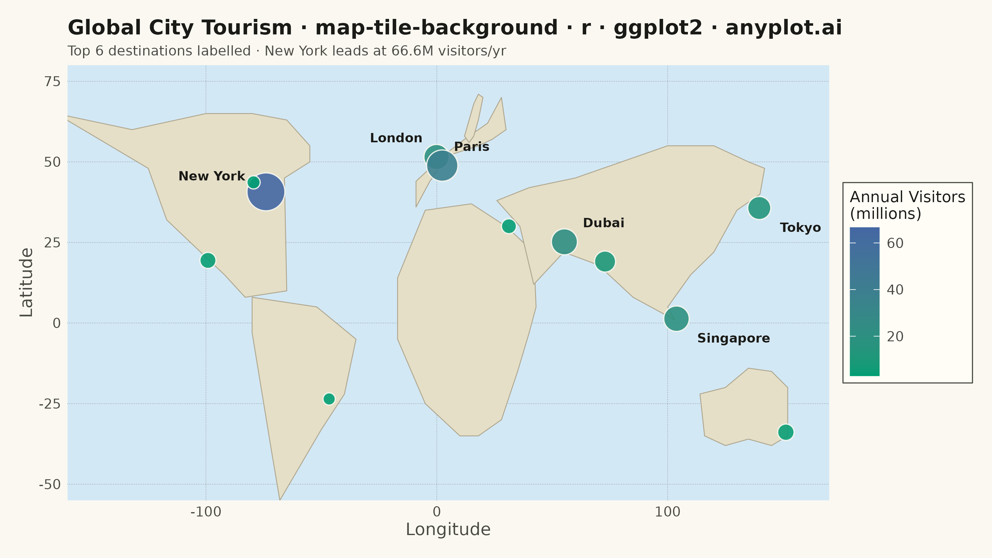
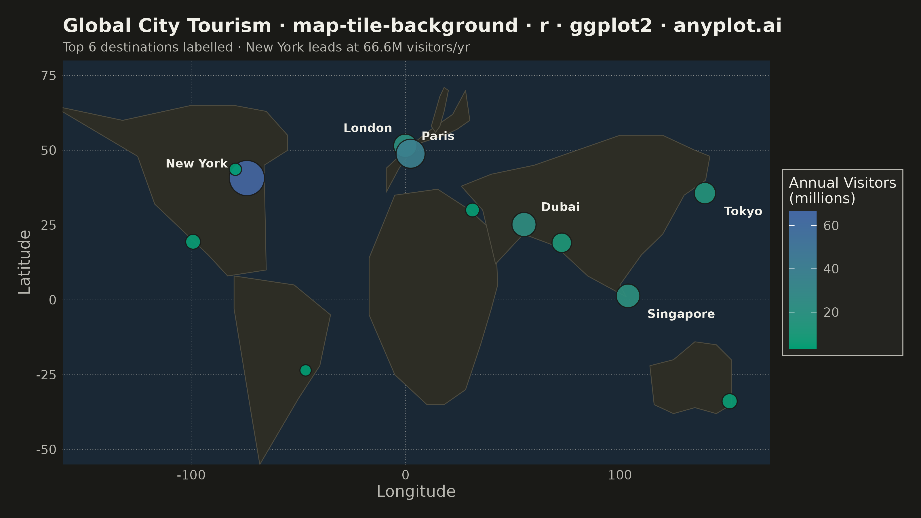
A map visualization that displays data points on top of tile-based backgrounds such as OpenStreetMap, Stamen, or satellite imagery. Unlike vector-based basemaps, tile backgrounds provide rich geographic context including street-level detail, terrain, or satellite imagery that loads dynamically as the user navigates. This visualization is essential for location-based analysis where real-world geographic context enhances data interpretation.
#' anyplot.ai
#' map-tile-background: Map with Tile Background
#' Library: ggplot2 3.5.1 | R 4.4.1
#' Quality: 84/100 | Created: 2026-05-27

library(ggplot2)
library(ragg)

set.seed(42)

# Theme tokens
THEME       <- Sys.getenv("ANYPLOT_THEME", "light")
PAGE_BG     <- if (THEME == "light") "#FAF8F1" else "#1A1A17"
ELEVATED_BG <- if (THEME == "light") "#FFFDF6" else "#242420"
INK         <- if (THEME == "light") "#1A1A17" else "#F0EFE8"
INK_SOFT    <- if (THEME == "light") "#4A4A44" else "#B8B7B0"

# Map surface colors (visualization area, not chrome)
OCEAN_BG    <- if (THEME == "light") "#D3E8F5" else "#1A2835"
LAND_FILL   <- if (THEME == "light") "#E5DFC8" else "#2D2D25"
LAND_BORDER <- if (THEME == "light") "#B0A890" else "#4E4C40"

# Simplified continental outlines (approximate shapes for geographic context)
continents <- rbind(
  data.frame(
    lon   = c(-165, -125, -117, -92, -83,  -65,  -66,  -55,  -55,  -65,  -80, -100, -132, -165),
    lat   = c(  65,   48,   32,  15,   8,   10,   45,   50,   55,   63,   65,   65,   60,   65),
    group = "north_america"
  ),
  data.frame(
    lon   = c( -80,  -52,  -35,  -40,  -50,  -68,  -72,  -80,  -80),
    lat   = c(   8,    5,   -5,  -22,  -33,  -55,  -38,   -3,    8),
    group = "south_america"
  ),
  data.frame(
    lon   = c( -9,  -9,   3,  12,  22,  28,  30,  24,  18,   5,  -3,  -9),
    lat   = c( 36,  44,  52,  57,  62,  70,  60,  57,  55,  52,  44,  36),
    group = "europe"
  ),
  data.frame(
    lon   = c( 14,  16,  18,  20,  18,  16,  14,  12,  14),
    lat   = c( 56,  58,  63,  70,  71,  68,  63,  58,  56),
    group = "scandinavia"
  ),
  data.frame(
    lon   = c( -5,  15,  30,  42,  43,  40,  35,  28,  18,  10,  -5, -17, -17,  -5),
    lat   = c( 35,  37,  30,  22,   5,  -3, -15, -30, -35, -35, -25,  -5,  14,  35),
    group = "africa"
  ),
  data.frame(
    lon   = c( 26,  40,  60,  80, 100, 120, 135, 142, 140, 130, 120, 110, 100, 103,  85,  70,  55,  42,  36,  26),
    lat   = c( 38,  42,  45,  50,  55,  55,  50,  48,  40,  35,  22,  15,   5,   1,   8,  18,  22,  12,  30,  38),
    group = "asia"
  ),
  data.frame(
    lon   = c(114, 116, 125, 135, 145, 152, 152, 145, 135, 125, 114),
    lat   = c(-22, -35, -38, -36, -38, -35, -20, -15, -14, -20, -22),
    group = "australia"
  )
)

# 12 major cities with annual international visitor counts (millions)
cities <- data.frame(
  city       = c("New York", "London", "Paris", "Tokyo", "Dubai",
                 "Singapore", "Sydney", "Mumbai", "Sao Paulo", "Toronto",
                 "Cairo", "Mexico City"),
  lon        = c(-74.01,  -0.13,   2.35, 139.69,  55.27,
                 103.82, 151.21,  72.88, -46.63, -79.38,
                  31.24, -99.13),
  lat        = c( 40.71,  51.51,  48.85,  35.69,  25.20,
                   1.35, -33.87,  19.08, -23.55,  43.65,
                  30.04,  19.43),
  visitors_m = c(66.6, 19.1, 38.0, 14.2, 21.3,
                 19.8,  4.7, 10.5,  3.0,  3.1,
                  3.7,  4.4)
)

# Label the top 6 cities (>= 14M visitors); hand-tuned nudges to avoid overlap
label_cities <- cities[cities$visitors_m >= 14, ]
label_cities$nudge_x <- c(-9,  -6,   5,   9,   8,   9)
label_cities$nudge_y <- c( 5,   6,   6,  -6,   6,  -6)
label_cities$hjust   <- c( 1,   1,   0,   0,   0,   0)

title_str  <- "Global City Tourism · map-tile-background · r · ggplot2 · anyplot.ai"
title_size <- max(8, round(12 * 67 / nchar(title_str)))

p <- ggplot() +
  geom_polygon(
    data      = continents,
    aes(x = lon, y = lat, group = group),
    fill      = LAND_FILL,
    color     = LAND_BORDER,
    linewidth = 0.25
  ) +
  geom_point(
    data   = cities,
    aes(x = lon, y = lat, fill = visitors_m, size = visitors_m),
    color  = PAGE_BG,
    shape  = 21,
    stroke = 0.5,
    alpha  = 0.9
  ) +
  geom_text(
    data     = label_cities,
    aes(x = lon + nudge_x, y = lat + nudge_y, label = city, hjust = hjust),
    color    = INK,
    size     = 2.6,
    fontface = "bold"
  ) +
  scale_fill_gradient(
    low  = "#009E73",
    high = "#4467A3",
    name = "Annual Visitors\n(millions)"
  ) +
  scale_size_continuous(
    range = c(3, 10),
    guide = "none"
  ) +
  coord_cartesian(
    xlim   = c(-160, 170),
    ylim   = c(-55, 80),
    expand = FALSE
  ) +
  labs(
    title    = title_str,
    subtitle = "Top 6 destinations labelled · New York leads at 66.6M visitors/yr",
    x        = "Longitude",
    y        = "Latitude"
  ) +
  theme_minimal(base_size = 8) +
  theme(
    plot.background   = element_rect(fill = PAGE_BG,     color = PAGE_BG),
    panel.background  = element_rect(fill = OCEAN_BG,    color = NA),
    panel.grid.major  = element_line(color = INK_SOFT,   linewidth = 0.12, linetype = "dotted"),
    panel.grid.minor  = element_blank(),
    panel.border      = element_blank(),
    axis.title        = element_text(color = INK_SOFT,   size = 10),
    axis.text         = element_text(color = INK_SOFT,   size = 8),
    plot.title        = element_text(color = INK,        size = title_size, face = "bold"),
    plot.subtitle     = element_text(color = INK_SOFT,   size = 8),
    legend.background = element_rect(fill = ELEVATED_BG, color = INK_SOFT, linewidth = 0.3),
    legend.text       = element_text(color = INK_SOFT,   size = 8),
    legend.title      = element_text(color = INK,        size = 9),
    legend.key        = element_rect(fill = NA,           color = NA),
    plot.margin       = unit(c(0.4, 0.4, 0.4, 0.4), "cm")
  )

ggsave(
  filename = sprintf("plot-%s.png", THEME),
  plot     = p,
  device   = ragg::agg_png,
  width    = 8,
  height   = 4.5,
  units    = "in",
  dpi      = 400
)
Runnable source as JSON, for any HTTP client: https://api.anyplot.ai/specs/map-tile-background/ggplot2/code. Any spec id and library id listed in llms-full.txt fit the same URL shape; every URL below is complete and callable.
{
  "spec_id": "map-tile-background",
  "language": "r",
  "library": "ggplot2",
  "page": "https://anyplot.ai/map-tile-background/r/ggplot2",
  "hub": "https://anyplot.ai/map-tile-background",
  "code_json": "https://api.anyplot.ai/specs/map-tile-background/ggplot2/code",
  "spec_json": "https://api.anyplot.ai/specs/map-tile-background",
  "render_light_png": "https://storage.googleapis.com/anyplot-images/plots/map-tile-background/r/ggplot2/plot-light.png",
  "render_dark_png": "https://storage.googleapis.com/anyplot-images/plots/map-tile-background/r/ggplot2/plot-dark.png",
  "quality_score": 84.0,
  "license": "MIT",
  "guide": "https://anyplot.ai/llms.txt"
}
Part of Map with Tile Background on anyplot.ai.