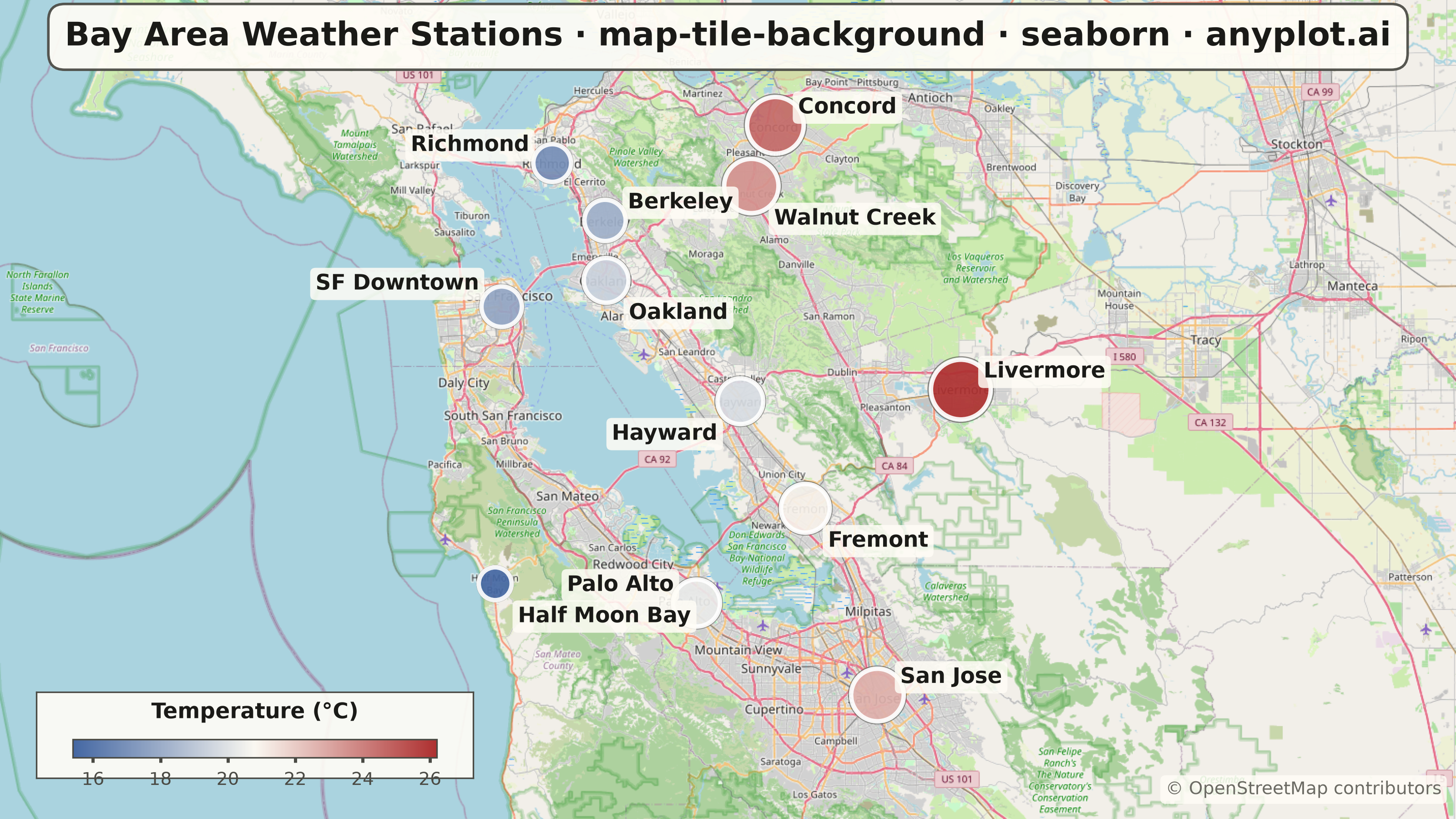
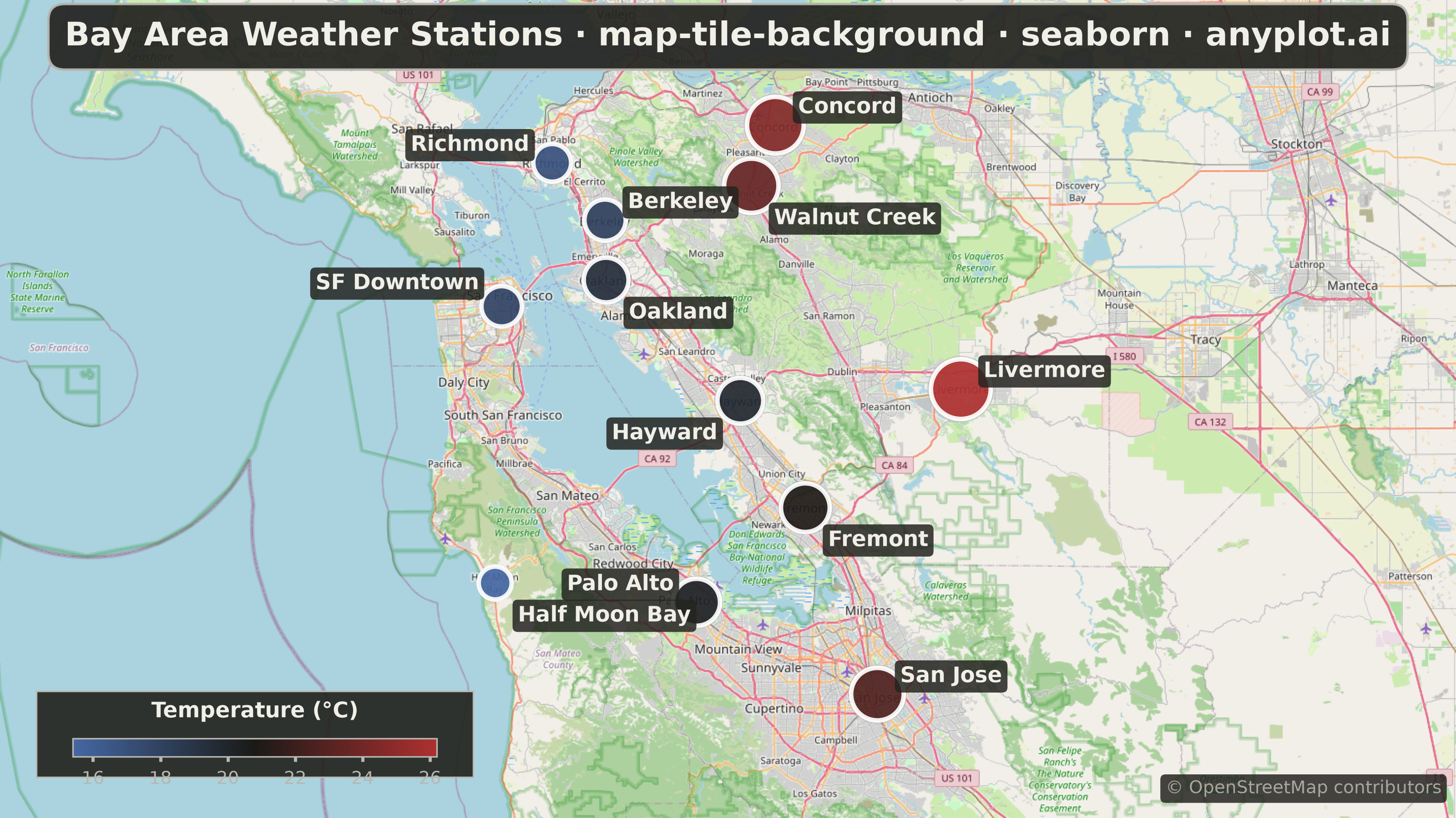
A map visualization that displays data points on top of tile-based backgrounds such as OpenStreetMap, Stamen, or satellite imagery. Unlike vector-based basemaps, tile backgrounds provide rich geographic context including street-level detail, terrain, or satellite imagery that loads dynamically as the user navigates. This visualization is essential for location-based analysis where real-world geographic context enhances data interpretation.
""" anyplot.ai
map-tile-background: Map with Tile Background
Library: seaborn 0.13.2 | Python 3.13.13
Quality: 89/100 | Updated: 2026-06-16
"""

import io
import os
import urllib.request

import matplotlib.pyplot as plt
import numpy as np
import pandas as pd
import seaborn as sns
from matplotlib.colors import LinearSegmentedColormap, Normalize
from PIL import Image


# Theme-adaptive chrome (see prompts/default-style-guide.md "Theme-adaptive Chrome")
THEME = os.getenv("ANYPLOT_THEME", "light")
PAGE_BG = "#FAF8F1" if THEME == "light" else "#1A1A17"
ELEVATED_BG = "#FFFDF6" if THEME == "light" else "#242420"
INK = "#1A1A17" if THEME == "light" else "#F0EFE8"
INK_SOFT = "#4A4A44" if THEME == "light" else "#B8B7B0"
INK_MUTED = "#6B6A63" if THEME == "light" else "#A8A79F"
MIDPOINT = "#FAF8F1" if THEME == "light" else "#1A1A17"

# Continuous data → Imprint diverging cmap, oriented cold-blue → neutral → hot-red
# so the temperature reads with the conventional hot→red / cold→blue mapping.
imprint_div = LinearSegmentedColormap.from_list("imprint_div", ["#4467A3", MIDPOINT, "#AE3030"])

# Data: a curated, well-spread set of Bay Area weather stations (avoids the dense
# southern cluster that caused label overlap in the previous attempt). Temperature
# encodes the Bay's coast-to-inland microclimate gradient.
np.random.seed(42)

stations_data = {
    "name": [
        "SF Downtown",
        "Oakland",
        "Berkeley",
        "Richmond",
        "Concord",
        "Walnut Creek",
        "Livermore",
        "Fremont",
        "Hayward",
        "Palo Alto",
        "San Jose",
        "Half Moon Bay",
    ],
    "lat": [37.7749, 37.8044, 37.8716, 37.9358, 37.9780, 37.9101, 37.6819, 37.5485, 37.6688, 37.4419, 37.3382, 37.4636],
    "lon": [
        -122.4194,
        -122.2712,
        -122.2727,
        -122.3477,
        -122.0311,
        -122.0652,
        -121.7680,
        -121.9886,
        -122.0808,
        -122.1430,
        -121.8863,
        -122.4286,
    ],
    "temperature": [17.8, 19.4, 18.1, 16.9, 24.6, 23.5, 26.2, 21.0, 19.8, 20.3, 22.7, 15.4],
    # Per-station label offset (points) + horizontal alignment, hand-tuned to
    # keep every label clear of its marker and of its neighbours.
    "off": [
        (-9, 9, "right"),
        (9, -13, "left"),
        (9, 7, "left"),
        (-9, 7, "right"),
        (9, 7, "left"),
        (9, -13, "left"),
        (9, 7, "left"),
        (9, -13, "left"),
        (-9, -13, "right"),
        (-9, 7, "right"),
        (9, 7, "left"),
        (9, -13, "left"),
    ],
}

df = pd.DataFrame(stations_data)

# --- Web Mercator tiling -----------------------------------------------------
ZOOM = 10  # city-level detail for a metro-area extent
TILE = 256
N = TILE * 2**ZOOM  # global pixel span at this zoom

# Web Mercator: project lon/lat → global-pixel coords. Inlined (vectorized numpy)
# to keep a flat, no-helper-functions structure; gx = (lon+180)/360·N,
# gy = (1 − asinh(tan(lat))/π)/2·N.
df["gx"] = (df["lon"] + 180.0) / 360.0 * N
df["gy"] = (1.0 - np.arcsinh(np.tan(np.radians(df["lat"]))) / np.pi) / 2.0 * N

# Padded data bounds in lon/lat, projected with the same formula, then expand to
# the 16:9 canvas aspect so the map fills the whole frame without distorting it.
pad_lon, pad_lat = 0.12, 0.14
wx0 = (df["lon"].min() - pad_lon + 180.0) / 360.0 * N
wx1 = (df["lon"].max() + pad_lon + 180.0) / 360.0 * N
wy_top = (1.0 - np.arcsinh(np.tan(np.radians(df["lat"].max() + pad_lat))) / np.pi) / 2.0 * N
wy_bot = (1.0 - np.arcsinh(np.tan(np.radians(df["lat"].min() - pad_lat))) / np.pi) / 2.0 * N
W, H = wx1 - wx0, wy_bot - wy_top
ASPECT = 16 / 9
if W / H < ASPECT:
    new_w = H * ASPECT
    cx = (wx0 + wx1) / 2
    wx0, wx1 = cx - new_w / 2, cx + new_w / 2
else:
    new_h = W / ASPECT
    cy = (wy_top + wy_bot) / 2
    wy_top, wy_bot = cy - new_h / 2, cy + new_h / 2

# Tiles covering the window
tx0, tx1 = int(wx0 // TILE), int((wx1 - 1) // TILE)
ty0, ty1 = int(wy_top // TILE), int((wy_bot - 1) // TILE)

stitched = Image.new("RGB", ((tx1 - tx0 + 1) * TILE, (ty1 - ty0 + 1) * TILE))
headers = {"User-Agent": "anyplot.ai/1.0 (educational visualization)"}
for tx in range(tx0, tx1 + 1):
    for ty in range(ty0, ty1 + 1):
        url = f"https://tile.openstreetmap.org/{ZOOM}/{tx}/{ty}.png"
        try:
            req = urllib.request.Request(url, headers=headers)
            with urllib.request.urlopen(req, timeout=10) as resp:
                tile = Image.open(io.BytesIO(resp.read())).convert("RGB")
        except Exception:
            tile = Image.new("RGB", (TILE, TILE), (224, 222, 214))
        stitched.paste(tile, ((tx - tx0) * TILE, (ty - ty0) * TILE))

# Crop the stitched mosaic to the exact 16:9 window (in global-pixel coords)
ox, oy = tx0 * TILE, ty0 * TILE
cropped = stitched.crop((int(round(wx0 - ox)), int(round(wy_top - oy)), int(round(wx1 - ox)), int(round(wy_bot - oy))))

# --- Plot --------------------------------------------------------------------
sns.set_theme(style="white", font_scale=1.0)

fig = plt.figure(figsize=(8, 4.5), dpi=400)  # → 3200 × 1800 px
fig.patch.set_facecolor(PAGE_BG)
ax = fig.add_axes([0, 0, 1, 1])  # full-bleed map
ax.set_axis_off()

ax.imshow(cropped, extent=[wx0, wx1, wy_bot, wy_top], aspect="auto", zorder=0)
ax.set_xlim(wx0, wx1)
ax.set_ylim(wy_bot, wy_top)

norm = Normalize(vmin=df["temperature"].min(), vmax=df["temperature"].max())

# Faint dark outer ring behind every marker. The white edge alone leaves the
# near-midpoint markers (off-white fill) low-contrast on the pale OSM tiles; this
# thin INK_SOFT ring guarantees a clean separation from the background for all
# temperatures. Sizes mirror seaborn's linear (170→560) size mapping, scaled up.
ring_size = 170 + (df["temperature"] - df["temperature"].min()) / (
    df["temperature"].max() - df["temperature"].min()
) * (560 - 170)
ax.scatter(
    df["gx"], df["gy"], s=ring_size * 1.16, facecolors="none", edgecolors=INK_SOFT, linewidths=0.9, alpha=0.6, zorder=2
)

sns.scatterplot(
    data=df,
    x="gx",
    y="gy",
    hue="temperature",
    size="temperature",
    sizes=(170, 560),
    palette=imprint_div,
    hue_norm=norm,
    edgecolor="white",
    linewidth=1.8,
    alpha=0.92,
    ax=ax,
    legend=False,
    zorder=3,
)

# Station labels with theme-adaptive callout boxes
for _, row in df.iterrows():
    dx, dy, ha = row["off"]
    ax.annotate(
        row["name"],
        (row["gx"], row["gy"]),
        xytext=(dx, dy),
        textcoords="offset points",
        fontsize=8.5,
        ha=ha,
        va="center",
        color=INK,
        fontweight="bold",
        bbox={"boxstyle": "round,pad=0.25", "facecolor": ELEVATED_BG, "edgecolor": "none", "alpha": 0.85},
        zorder=4,
    )

# Title banner (overlaid on the full-bleed map, theme-adaptive box)
title = "Bay Area Weather Stations · map-tile-background · seaborn · anyplot.ai"
ax.text(
    0.5,
    0.955,
    title,
    transform=ax.transAxes,
    ha="center",
    va="center",
    fontsize=round(14 * 67 / len(title)),
    fontweight="bold",
    color=INK,
    bbox={"boxstyle": "round,pad=0.5", "facecolor": ELEVATED_BG, "edgecolor": INK_SOFT, "alpha": 0.93},
    zorder=6,
)

# Colorbar in a translucent panel, bottom-left (over Pacific water — no markers there)
panel = ax.inset_axes([0.025, 0.05, 0.30, 0.105], zorder=5)
panel.set_facecolor(ELEVATED_BG)
panel.patch.set_alpha(0.92)
panel.set_xticks([])
panel.set_yticks([])
for spine in panel.spines.values():
    spine.set_edgecolor(INK_SOFT)
    spine.set_linewidth(0.6)

cax = ax.inset_axes([0.05, 0.075, 0.25, 0.022], zorder=6)
sm = plt.cm.ScalarMappable(cmap=imprint_div, norm=norm)
sm.set_array([])
cbar = fig.colorbar(sm, cax=cax, orientation="horizontal")
cbar.outline.set_edgecolor(INK_SOFT)
cbar.outline.set_linewidth(0.6)
cbar.ax.tick_params(labelsize=7, color=INK_SOFT, labelcolor=INK_SOFT, length=2)
ax.text(
    0.175,
    0.13,
    "Temperature (°C)",
    transform=ax.transAxes,
    ha="center",
    va="center",
    fontsize=8.5,
    fontweight="bold",
    color=INK,
    zorder=7,
)

# OpenStreetMap attribution (required by license), bottom-right
ax.text(
    0.99,
    0.025,
    "© OpenStreetMap contributors",
    transform=ax.transAxes,
    ha="right",
    va="bottom",
    fontsize=7,
    color=INK_MUTED,
    bbox={"boxstyle": "round,pad=0.3", "facecolor": ELEVATED_BG, "edgecolor": "none", "alpha": 0.85},
    zorder=6,
)

plt.savefig(f"plot-{THEME}.png", dpi=400, facecolor=PAGE_BG)
Runnable source as JSON, for any HTTP client: https://api.anyplot.ai/specs/map-tile-background/seaborn/code. Any spec id and library id listed in llms-full.txt fit the same URL shape; every URL below is complete and callable.
{
  "spec_id": "map-tile-background",
  "language": "python",
  "library": "seaborn",
  "page": "https://anyplot.ai/map-tile-background/python/seaborn",
  "hub": "https://anyplot.ai/map-tile-background",
  "code_json": "https://api.anyplot.ai/specs/map-tile-background/seaborn/code",
  "spec_json": "https://api.anyplot.ai/specs/map-tile-background",
  "render_light_png": "https://storage.googleapis.com/anyplot-images/plots/map-tile-background/python/seaborn/plot-light.png",
  "render_dark_png": "https://storage.googleapis.com/anyplot-images/plots/map-tile-background/python/seaborn/plot-dark.png",
  "quality_score": 89.0,
  "license": "MIT",
  "guide": "https://anyplot.ai/llms.txt"
}
Part of Map with Tile Background on anyplot.ai.