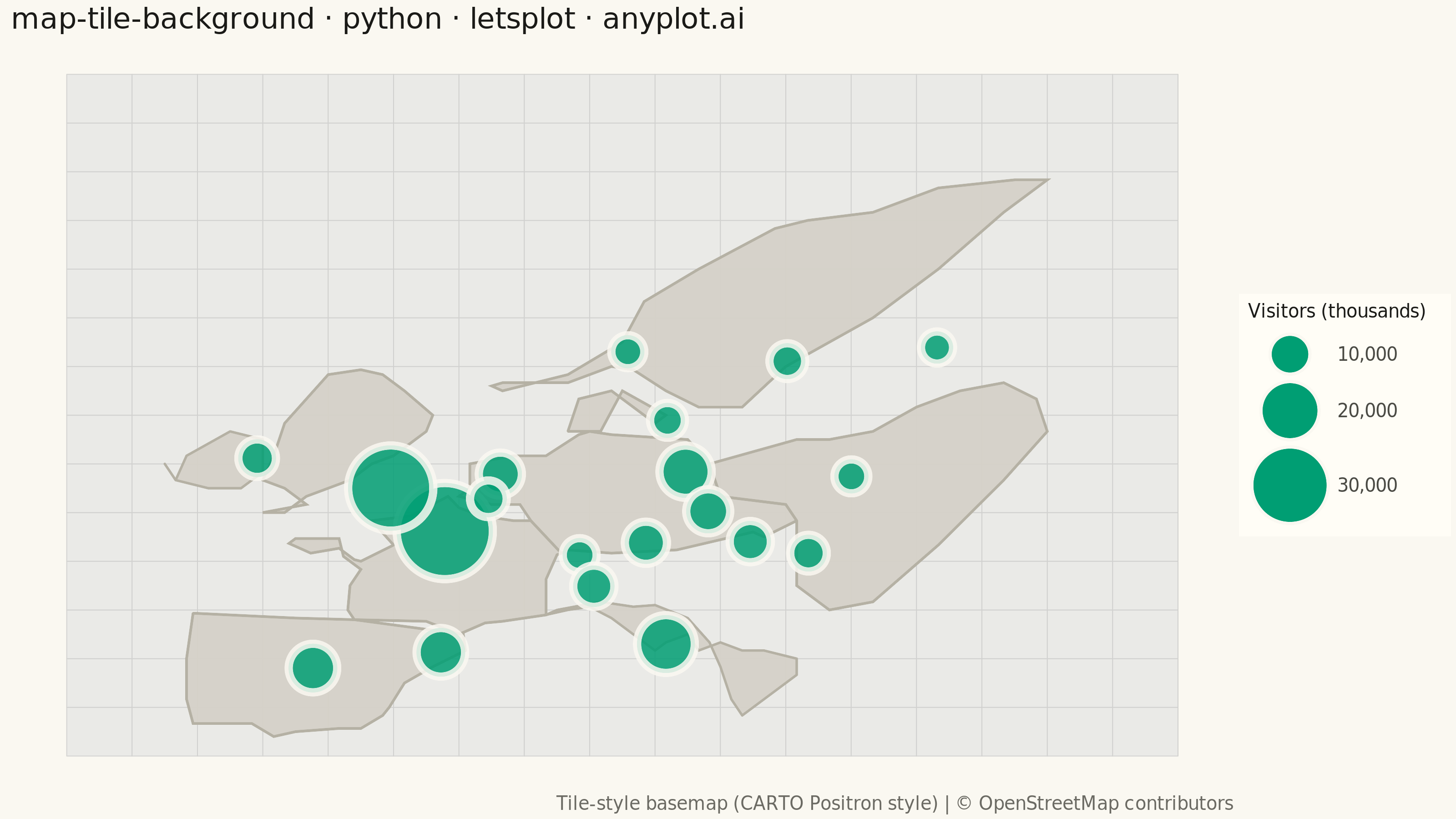
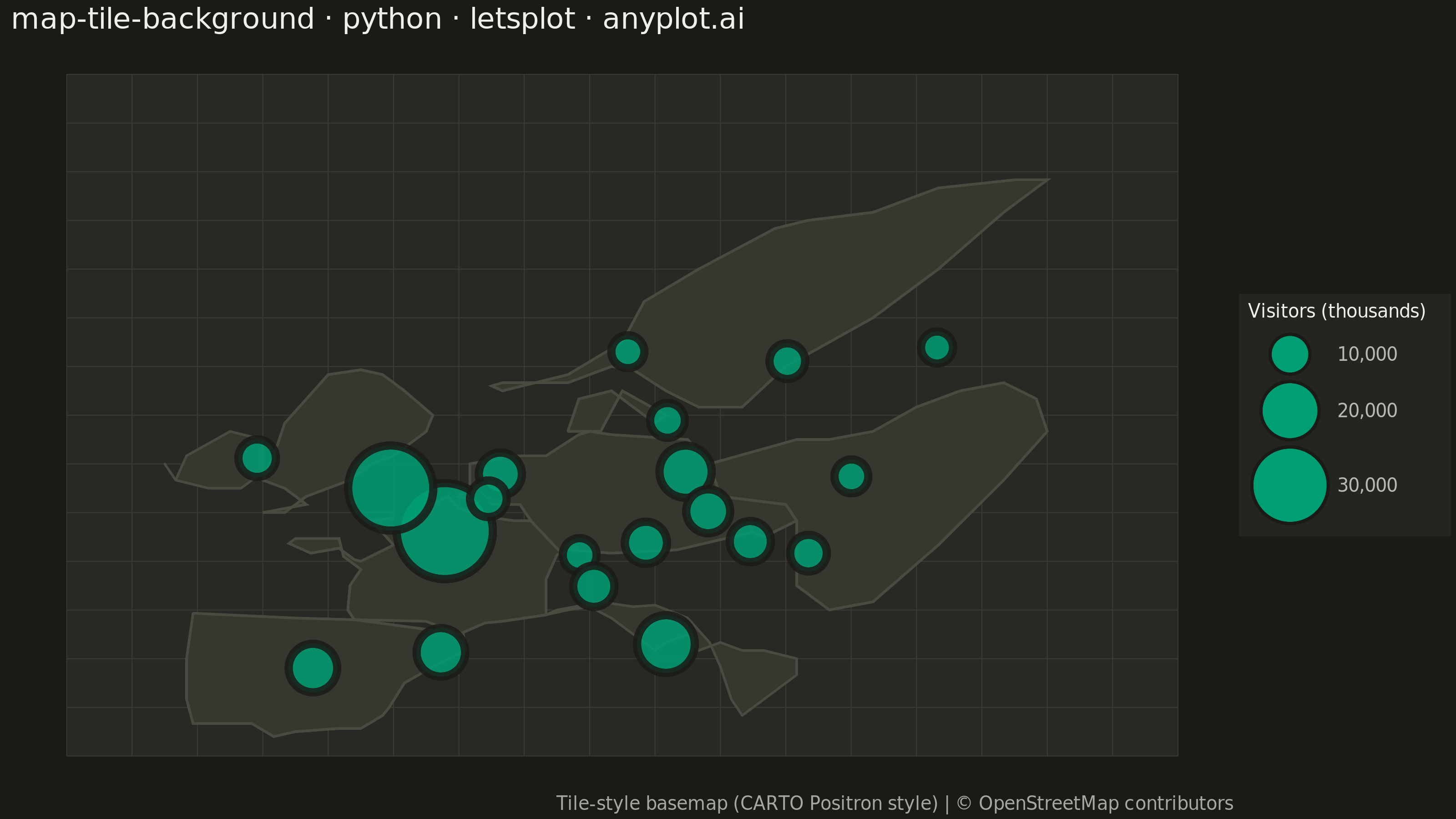
A map visualization that displays data points on top of tile-based backgrounds such as OpenStreetMap, Stamen, or satellite imagery. Unlike vector-based basemaps, tile backgrounds provide rich geographic context including street-level detail, terrain, or satellite imagery that loads dynamically as the user navigates. This visualization is essential for location-based analysis where real-world geographic context enhances data interpretation.
""" anyplot.ai
map-tile-background: Map with Tile Background
Library: letsplot 4.10.1 | Python 3.13.13
Quality: 91/100 | Updated: 2026-05-27
"""
import os
import pandas as pd
from lets_plot import (
LetsPlot,
aes,
element_rect,
element_text,
geom_livemap,
geom_point,
geom_polygon,
geom_rect,
ggplot,
ggsize,
labs,
layer_tooltips,
scale_size,
theme,
theme_void,
tilesets,
)
from lets_plot.export import ggsave
LetsPlot.setup_html()
THEME = os.getenv("ANYPLOT_THEME", "light")
PAGE_BG = "#FAF8F1" if THEME == "light" else "#1A1A17"
ELEVATED_BG = "#FFFDF6" if THEME == "light" else "#242420"
INK = "#1A1A17" if THEME == "light" else "#F0EFE8"
INK_SOFT = "#4A4A44" if THEME == "light" else "#B8B7B0"
INK_MUTED = "#6B6A63" if THEME == "light" else "#A8A79F"
BRAND = "#009E73" # Imprint palette position 1 — ALWAYS first series
# Tile and land polygon colors adapt to theme
TILE_BG = "#E8E8E6" if THEME == "light" else "#2A2A27"
TILE_BORDER = "#D0D0CE" if THEME == "light" else "#3A3A37"
LAND_FILL = "#D5D1C8" if THEME == "light" else "#38382F"
LAND_BORDER = "#B5B1A4" if THEME == "light" else "#4A4A40"
# Data: European cities with annual visitor counts (thousands)
cities_data = {
"city": [
"Paris",
"London",
"Berlin",
"Rome",
"Madrid",
"Amsterdam",
"Vienna",
"Prague",
"Barcelona",
"Munich",
"Brussels",
"Zurich",
"Milan",
"Dublin",
"Copenhagen",
"Stockholm",
"Oslo",
"Helsinki",
"Warsaw",
"Budapest",
],
"lat": [
48.86,
51.51,
52.52,
41.90,
40.42,
52.37,
48.21,
50.08,
41.39,
48.14,
50.85,
47.38,
45.46,
53.35,
55.68,
59.33,
59.91,
60.17,
52.23,
47.50,
],
"lon": [
2.35,
-0.13,
13.40,
12.50,
-3.70,
4.90,
16.37,
14.44,
2.17,
11.58,
4.35,
8.54,
9.19,
-6.26,
12.57,
18.07,
10.75,
24.94,
21.01,
19.04,
],
"visitors": [
38000,
32000,
14000,
17000,
12000,
9000,
8000,
9500,
12000,
8500,
5500,
4000,
8000,
6000,
4500,
5000,
3500,
3000,
4000,
5500,
],
}
df = pd.DataFrame(cities_data)
TITLE = "map-tile-background · python · letsplot · anyplot.ai"
# Interactive HTML version — geom_livemap with real tile provider
map_tiles = tilesets.LETS_PLOT_DARK if THEME == "dark" else tilesets.CARTO_POSITRON
plot_interactive = (
ggplot()
+ geom_livemap(location=[-12, 35, 32, 72], zoom=4, tiles=map_tiles)
+ geom_point(
aes(x="lon", y="lat", size="visitors"),
data=df,
fill=BRAND,
color=PAGE_BG,
alpha=0.85,
shape=21,
stroke=2,
tooltips=layer_tooltips().title("@city").line("Visitors|@visitors K/year"),
)
+ scale_size(range=[6, 22], name="Visitors (thousands)")
+ labs(title=TITLE)
+ ggsize(800, 450)
+ theme(
plot_title=element_text(size=16, color=INK),
legend_title=element_text(size=10, color=INK),
legend_text=element_text(size=10, color=INK_SOFT),
legend_background=element_rect(fill=ELEVATED_BG),
plot_background=element_rect(fill=PAGE_BG, color=PAGE_BG),
legend_position="right",
)
)
ggsave(plot_interactive, f"plot-{THEME}.html", path=".")
# Static PNG version — simulated tile-style background for raster export
tiles_rows = []
tile_size = 3
for lon_val in range(-15, 35, tile_size):
for lat_val in range(35, 75, tile_size):
tiles_rows.append({"xmin": lon_val, "xmax": lon_val + tile_size, "ymin": lat_val, "ymax": lat_val + tile_size})
df_tiles = pd.DataFrame(tiles_rows)
# European landmass polygons — per-country outlines for recognizable geography
# France (includes Breton peninsula; ~29 vertices)
france = pd.DataFrame(
{
"lon": [
-1.8,
-2.1,
-2.0,
-1.5,
-2.3,
-2.5,
-4.5,
-4.8,
-3.8,
-2.5,
-1.8,
-1.5,
0.0,
-1.0,
0.8,
2.5,
3.0,
4.0,
5.5,
6.3,
7.7,
7.5,
7.0,
7.0,
5.0,
4.2,
3.0,
1.5,
-1.8,
],
"lat": [
43.4,
44.0,
45.5,
46.5,
47.3,
48.4,
48.4,
48.1,
47.5,
47.8,
47.1,
47.0,
48.0,
49.5,
49.8,
51.0,
50.3,
49.8,
49.5,
49.5,
47.5,
47.4,
45.9,
43.7,
43.3,
43.2,
42.5,
43.3,
43.4,
],
"region": ["France"] * 29,
}
)
# Iberian Peninsula — Spain + Portugal (~21 vertices)
iberia = pd.DataFrame(
{
"lon": [
-9.2,
-7.5,
-4.5,
-1.8,
3.2,
3.3,
1.8,
0.5,
-0.2,
-0.5,
-1.5,
-2.5,
-4.5,
-5.5,
-6.5,
-7.5,
-8.8,
-9.2,
-9.5,
-9.5,
-9.2,
],
"lat": [
43.8,
43.7,
43.5,
43.4,
42.5,
41.5,
40.5,
39.5,
38.0,
37.5,
36.7,
36.7,
36.5,
36.2,
37.0,
37.0,
37.0,
37.0,
38.5,
41.0,
43.8,
],
"region": ["Iberia"] * 21,
}
)
# Central Europe — Germany, Netherlands, Belgium, Austria, Czech, Slovakia (~24 vertices)
central_europe = pd.DataFrame(
{
"lon": [
6.3,
7.7,
8.0,
10.0,
13.0,
15.5,
16.5,
17.0,
18.5,
18.0,
15.0,
14.5,
13.5,
10.0,
9.0,
8.5,
7.0,
5.5,
3.5,
3.5,
3.0,
4.5,
5.8,
6.3,
],
"lat": [
49.5,
47.5,
47.7,
47.5,
47.7,
48.5,
48.8,
48.5,
49.5,
50.5,
51.0,
53.0,
54.5,
54.8,
55.0,
54.8,
53.5,
53.5,
53.0,
51.5,
51.0,
50.5,
50.5,
49.5,
],
"region": ["Central_EU"] * 24,
}
)
# Eastern Europe — Poland, Balkans, Romania, Hungary, Ukraine west (~18 vertices)
eastern_europe = pd.DataFrame(
{
"lon": [
18.5,
18.0,
15.0,
14.5,
18.5,
20.0,
22.0,
24.0,
26.0,
28.0,
29.5,
30.0,
28.0,
25.0,
22.0,
20.0,
18.5,
18.5,
],
"lat": [
49.5,
50.5,
51.0,
53.0,
54.5,
54.5,
55.0,
56.5,
57.5,
58.0,
57.0,
55.0,
52.0,
48.0,
44.5,
44.0,
45.5,
49.5,
],
"region": ["Eastern_EU"] * 18,
}
)
# Scandinavia — Norway + Sweden peninsula (~25 vertices)
scandinavia = pd.DataFrame(
{
"lon": [
5.0,
8.0,
10.0,
11.0,
12.5,
14.0,
16.0,
18.0,
20.0,
22.0,
25.0,
28.0,
30.0,
28.5,
25.0,
22.0,
19.0,
17.5,
14.0,
11.5,
10.5,
8.0,
5.0,
4.5,
5.0,
],
"lat": [
58.0,
58.0,
59.0,
58.8,
57.5,
56.5,
56.5,
59.0,
60.5,
62.0,
65.0,
68.5,
70.5,
70.5,
70.0,
68.5,
68.0,
67.5,
65.0,
63.0,
60.5,
58.5,
57.5,
57.8,
58.0,
],
"region": ["Scandinavia"] * 25,
}
)
# Great Britain (~20 vertices)
britain = pd.DataFrame(
{
"lon": [
-6.0,
-5.0,
-4.0,
-3.0,
-2.0,
-1.0,
0.0,
1.5,
1.8,
0.5,
-0.5,
-1.5,
-3.0,
-4.0,
-5.0,
-5.5,
-6.0,
-5.0,
-4.0,
-6.0,
],
"lat": [
50.0,
50.0,
51.0,
51.5,
52.0,
53.0,
53.5,
55.0,
56.0,
57.5,
58.5,
58.8,
58.5,
57.0,
55.5,
53.5,
52.0,
51.5,
50.5,
50.0,
],
"region": ["Britain"] * 20,
}
)
# Ireland (~10 vertices)
ireland = pd.DataFrame(
{
"lon": [-10.0, -9.5, -7.5, -6.0, -6.0, -7.0, -8.5, -10.0, -10.5, -10.0],
"lat": [52.0, 53.5, 55.0, 54.5, 52.5, 51.5, 51.5, 52.0, 53.0, 52.0],
"region": ["Ireland"] * 10,
}
)
# Italy — boot shape (~26 vertices)
italy = pd.DataFrame(
{
"lon": [
7.0,
7.5,
9.5,
11.0,
12.0,
13.5,
14.5,
15.0,
15.5,
16.0,
16.5,
18.5,
18.5,
17.0,
16.0,
15.0,
14.0,
13.5,
12.5,
12.0,
11.0,
10.0,
9.0,
8.0,
7.0,
7.0,
],
"lat": [
43.7,
44.0,
44.5,
44.2,
44.3,
43.5,
42.0,
40.5,
38.5,
37.5,
38.0,
40.0,
41.0,
41.5,
41.5,
42.0,
41.5,
42.5,
42.0,
41.5,
42.5,
43.5,
44.2,
44.0,
43.7,
43.7,
],
"region": ["Italy"] * 26,
}
)
# Denmark (~8 vertices)
denmark = pd.DataFrame(
{
"lon": [8.0, 9.5, 10.5, 12.5, 12.0, 10.0, 8.5, 8.0],
"lat": [55.0, 55.0, 57.5, 56.0, 55.5, 57.5, 57.0, 55.0],
"region": ["Denmark"] * 8,
}
)
df_land = pd.concat(
[france, iberia, central_europe, eastern_europe, scandinavia, britain, ireland, italy, denmark], ignore_index=True
)
plot_static = (
ggplot()
+ geom_rect(
aes(xmin="xmin", xmax="xmax", ymin="ymin", ymax="ymax"),
data=df_tiles,
fill=TILE_BG,
color=TILE_BORDER,
size=0.2,
alpha=0.9,
)
+ geom_polygon(
aes(x="lon", y="lat", group="region"), data=df_land, fill=LAND_FILL, color=LAND_BORDER, size=0.6, alpha=0.95
)
+ geom_point(
aes(x="lon", y="lat", size="visitors"), data=df, fill=BRAND, color=PAGE_BG, alpha=0.85, shape=21, stroke=2
)
+ scale_size(range=[6, 22], name="Visitors (thousands)")
+ labs(title=TITLE, caption="Tile-style basemap (CARTO Positron style) | © OpenStreetMap contributors")
+ ggsize(800, 450)
+ theme_void()
+ theme(
plot_title=element_text(size=16, color=INK),
plot_caption=element_text(size=10, color=INK_MUTED),
legend_title=element_text(size=10, color=INK),
legend_text=element_text(size=10, color=INK_SOFT),
legend_background=element_rect(fill=ELEVATED_BG, color=INK_SOFT),
legend_position="right",
plot_background=element_rect(fill=PAGE_BG, color=PAGE_BG),
)
)
ggsave(plot_static, f"plot-{THEME}.png", path=".", scale=4)
Runnable source as JSON, for any HTTP client: https://api.anyplot.ai/specs/map-tile-background/letsplot/code. Any spec id and library id listed in llms-full.txt fit the same URL shape; every URL below is complete and callable.
{
  "spec_id": "map-tile-background",
  "language": "python",
  "library": "letsplot",
  "page": "https://anyplot.ai/map-tile-background/python/letsplot",
  "hub": "https://anyplot.ai/map-tile-background",
  "code_json": "https://api.anyplot.ai/specs/map-tile-background/letsplot/code",
  "spec_json": "https://api.anyplot.ai/specs/map-tile-background",
  "render_light_png": "https://storage.googleapis.com/anyplot-images/plots/map-tile-background/python/letsplot/plot-light.png",
  "render_dark_png": "https://storage.googleapis.com/anyplot-images/plots/map-tile-background/python/letsplot/plot-dark.png",
  "interactive_light_html": "https://storage.googleapis.com/anyplot-images/plots/map-tile-background/python/letsplot/plot-light.html",
  "interactive_dark_html": "https://storage.googleapis.com/anyplot-images/plots/map-tile-background/python/letsplot/plot-dark.html",
  "quality_score": 91.0,
  "license": "MIT",
  "guide": "https://anyplot.ai/llms.txt"
}
Part of Map with Tile Background on anyplot.ai.