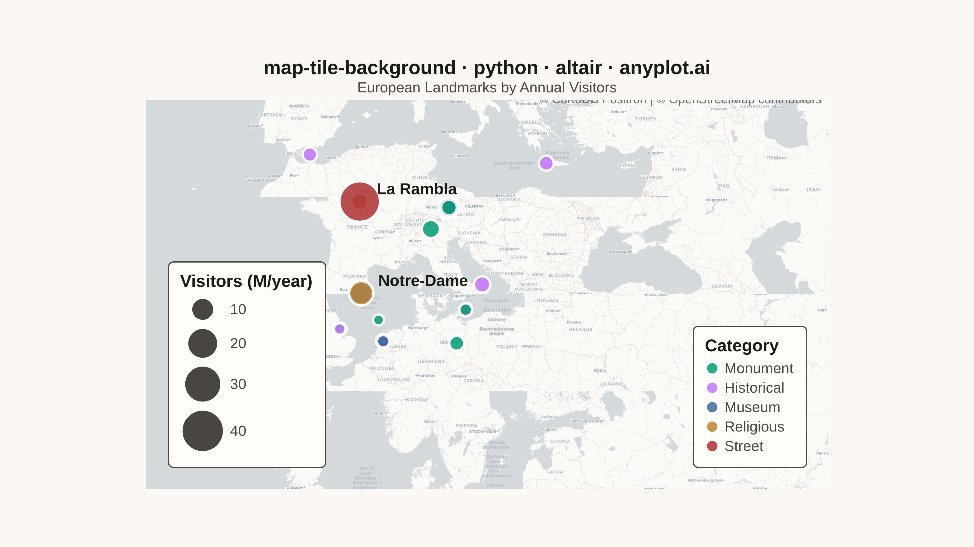
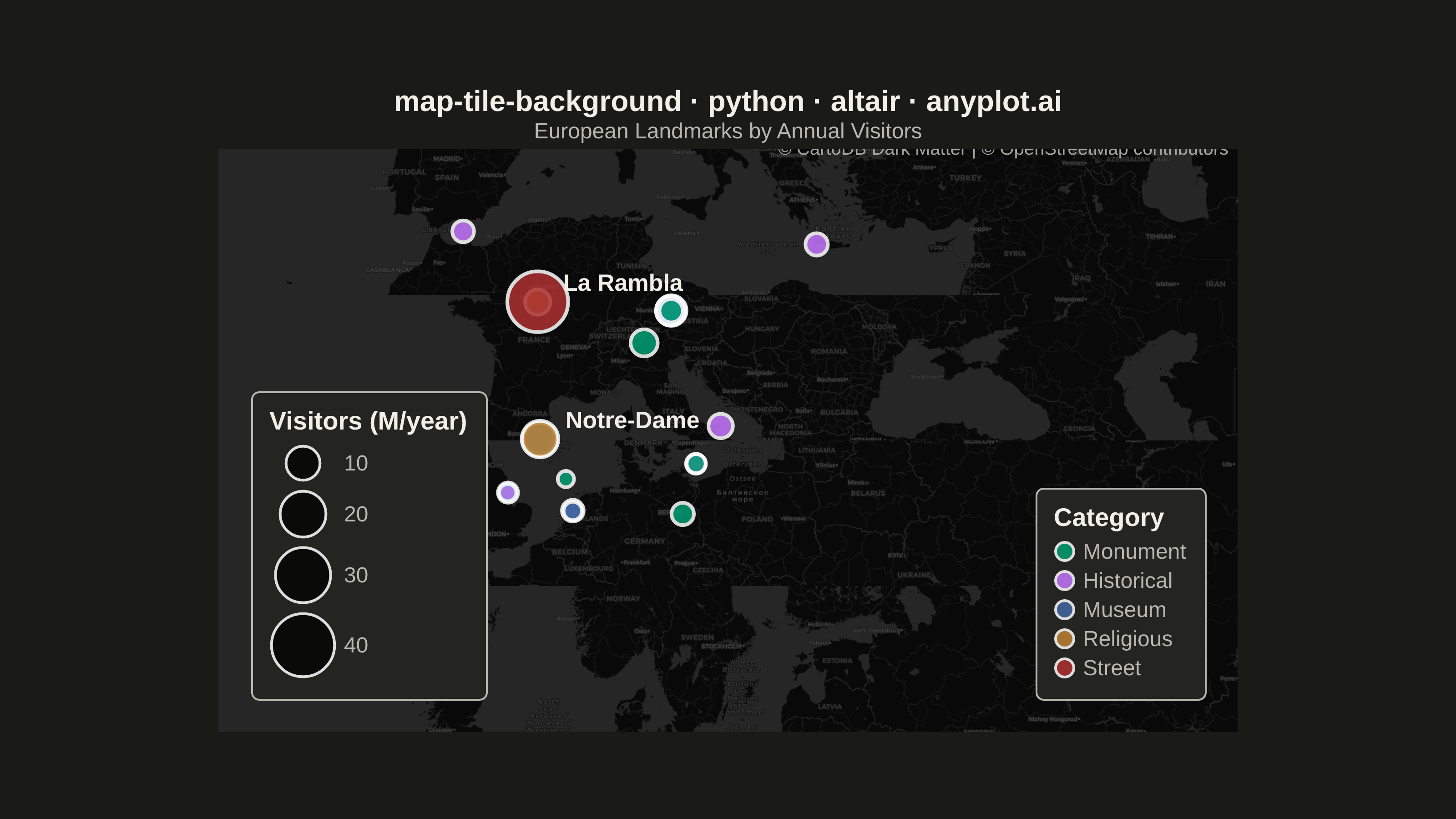
A map visualization that displays data points on top of tile-based backgrounds such as OpenStreetMap, Stamen, or satellite imagery. Unlike vector-based basemaps, tile backgrounds provide rich geographic context including street-level detail, terrain, or satellite imagery that loads dynamically as the user navigates. This visualization is essential for location-based analysis where real-world geographic context enhances data interpretation.
""" anyplot.ai
map-tile-background: Map with Tile Background
Library: altair 6.1.0 | Python 3.13.13
Quality: 84/100 | Updated: 2026-05-27
"""

import os
import sys


# Work around filename shadowing the altair library
sys.path.pop(0)

import altair as alt
import numpy as np
import pandas as pd
from PIL import Image


# Theme
THEME = os.getenv("ANYPLOT_THEME", "light")
PAGE_BG = "#FAF8F1" if THEME == "light" else "#1A1A17"
ELEVATED_BG = "#FFFDF6" if THEME == "light" else "#242420"
INK = "#1A1A17" if THEME == "light" else "#F0EFE8"
INK_SOFT = "#4A4A44" if THEME == "light" else "#B8B7B0"
INK_MUTED = "#6B6A63" if THEME == "light" else "#A8A79F"

IMPRINT_PALETTE = ["#009E73", "#C475FD", "#4467A3", "#BD8233", "#AE3030", "#2ABCCD", "#954477", "#99B314"]

# Data: European landmarks with visitor counts (millions annually)
np.random.seed(42)

landmarks = {
    "name": [
        "Eiffel Tower",
        "Colosseum",
        "Sagrada Familia",
        "Big Ben",
        "Rijksmuseum",
        "Brandenburg Gate",
        "Prague Castle",
        "Schonbrunn Palace",
        "Louvre Museum",
        "Vatican Museums",
        "Alhambra",
        "Buckingham Palace",
        "Anne Frank House",
        "Acropolis",
        "Charles Bridge",
        "Manneken Pis",
        "Tower of Pisa",
        "Notre-Dame",
        "Trevi Fountain",
        "La Rambla",
    ],
    "lat": [
        48.8584,
        41.8902,
        41.4036,
        51.5007,
        52.3600,
        52.5163,
        50.0911,
        48.1845,
        48.8606,
        41.9065,
        37.1760,
        51.5014,
        52.3752,
        37.9715,
        50.0865,
        50.8450,
        43.7230,
        48.8530,
        41.9009,
        41.3809,
    ],
    "lon": [
        2.2945,
        12.4922,
        2.1744,
        -0.1246,
        4.8852,
        13.3777,
        14.4006,
        16.3122,
        2.3376,
        12.4536,
        -3.5881,
        -0.1419,
        4.8840,
        23.7257,
        14.4114,
        4.3499,
        10.3966,
        2.3499,
        12.4833,
        2.1734,
    ],
    "visitors": [7.0, 7.6, 4.5, 2.0, 2.7, 3.0, 1.9, 4.0, 9.6, 6.9, 2.7, 0.8, 1.3, 3.0, 1.5, 0.5, 5.5, 12.0, 3.5, 37.0],
    "category": [
        "Monument",
        "Historical",
        "Religious",
        "Monument",
        "Museum",
        "Monument",
        "Historical",
        "Historical",
        "Museum",
        "Museum",
        "Historical",
        "Historical",
        "Museum",
        "Historical",
        "Monument",
        "Monument",
        "Monument",
        "Religious",
        "Monument",
        "Street",
    ],
}

df = pd.DataFrame(landmarks)

# Tile grid: 7 wide × 4 tall gives 1.75:1 aspect ≈ 16:9 landscape
zoom = 5
tx_min, tx_max = 14, 20  # 7 tiles wide (lon ≈ −22° to 56°)
ty_min, ty_max = 9, 12  # 4 tiles tall (lat ≈ 32° to 62°)

n_tiles_x = tx_max - tx_min + 1  # 7
n_tiles_y = ty_max - ty_min + 1  # 4

# Inner view: 560×320; tile_disp = 80 each (square tiles — no Mercator distortion)
chart_width = 560
chart_height = 320
tile_disp_w = chart_width / n_tiles_x  # 80.0
tile_disp_h = chart_height / n_tiles_y  # 80.0

# Web Mercator projection: lon/lat → pixel coords within the chart
df["tile_x"] = (df["lon"] + 180) / 360 * (2**zoom)
df["lat_rad"] = np.radians(df["lat"])
df["tile_y"] = (1 - np.log(np.tan(df["lat_rad"]) + 1 / np.cos(df["lat_rad"])) / np.pi) / 2 * (2**zoom)
df["x_pix"] = (df["tile_x"] - tx_min) * tile_disp_w
df["y_pix"] = (df["tile_y"] - ty_min) * tile_disp_h

df = df[(df["x_pix"] >= 0) & (df["x_pix"] <= chart_width) & (df["y_pix"] >= 0) & (df["y_pix"] <= chart_height)]

# Tile provider: CartoDB Positron (light, muted) or CartoDB Dark Matter (dark)
# Demonstrates multiple tile provider support per spec; muted basemap lets anyplot colors pop
if THEME == "dark":
    tile_base_url = "https://basemaps.cartocdn.com/dark_all"
    tile_provider = "CartoDB Dark Matter"
else:
    tile_base_url = "https://basemaps.cartocdn.com/light_all"
    tile_provider = "CartoDB Positron"

# Build tile grid for mark_image
tiles = []
for tx in range(tx_min, tx_max + 1):
    for ty in range(ty_min, ty_max + 1):
        tiles.append(
            {
                "url": f"{tile_base_url}/{zoom}/{tx}/{ty}.png",
                "x": (tx - tx_min + 0.5) * tile_disp_w,
                "y": (ty - ty_min + 0.5) * tile_disp_h,
            }
        )
tiles_df = pd.DataFrame(tiles)

# Layer 1: CartoDB tile background (Positron in light, Dark Matter in dark)
tile_layer = (
    alt.Chart(tiles_df)
    .mark_image(width=tile_disp_w, height=tile_disp_h)
    .encode(
        url="url:N",
        x=alt.X("x:Q", scale=alt.Scale(domain=[0, chart_width], nice=False), axis=None),
        y=alt.Y("y:Q", scale=alt.Scale(domain=[0, chart_height], nice=False), axis=None),
    )
)

# Category → Imprint palette (canonical positions 1-5)
category_colors = {
    "Monument": IMPRINT_PALETTE[0],  # #009E73 green
    "Historical": IMPRINT_PALETTE[1],  # #C475FD lavender
    "Museum": IMPRINT_PALETTE[2],  # #4467A3 blue
    "Religious": IMPRINT_PALETTE[3],  # #BD8233 ochre
    "Street": IMPRINT_PALETTE[4],  # #AE3030 red
}

# Layer 2: landmark circles sized by visitors
points_layer = (
    alt.Chart(df)
    .mark_circle(opacity=0.85, stroke="#FFFFFF", strokeWidth=2)
    .encode(
        x=alt.X("x_pix:Q", scale=alt.Scale(domain=[0, chart_width], nice=False), axis=None),
        y=alt.Y("y_pix:Q", scale=alt.Scale(domain=[0, chart_height], nice=False), axis=None),
        size=alt.Size(
            "visitors:Q",
            scale=alt.Scale(domain=[0.5, 40], range=[80, 1200]),
            legend=alt.Legend(
                title="Visitors (M/year)", titleFontSize=14, labelFontSize=12, orient="bottom-left", tickCount=4
            ),
        ),
        color=alt.Color(
            "category:N",
            scale=alt.Scale(domain=list(category_colors.keys()), range=list(category_colors.values())),
            legend=alt.Legend(title="Category", titleFontSize=14, labelFontSize=12, orient="bottom-right"),
        ),
        tooltip=[
            alt.Tooltip("name:N", title="Landmark"),
            alt.Tooltip("visitors:Q", title="Visitors (M)", format=".1f"),
            alt.Tooltip("category:N", title="Category"),
        ],
    )
)

# Layer 3: labels for top landmarks (≥10M threshold avoids cluster overlap)
labels_df = df[df["visitors"] >= 10].copy()
labels_layer = (
    alt.Chart(labels_df)
    .mark_text(align="left", dx=14, dy=-10, fontSize=13, fontWeight="bold", color=INK)
    .encode(
        x=alt.X("x_pix:Q", scale=alt.Scale(domain=[0, chart_width], nice=False), axis=None),
        y=alt.Y("y_pix:Q", scale=alt.Scale(domain=[0, chart_height], nice=False), axis=None),
        text="name:N",
    )
)

# Layer 4: tile provider attribution (required by CartoDB and OSM license)
attribution_df = pd.DataFrame(
    {"text": [f"© {tile_provider} | © OpenStreetMap contributors"], "x": [chart_width - 5], "y": [chart_height - 5]}
)
attribution_layer = (
    alt.Chart(attribution_df)
    .mark_text(align="right", baseline="bottom", fontSize=10, color=INK_MUTED)
    .encode(
        x=alt.X("x:Q", scale=alt.Scale(domain=[0, chart_width], nice=False), axis=None),
        y=alt.Y("y:Q", scale=alt.Scale(domain=[0, chart_height], nice=False), axis=None),
        text="text:N",
    )
)

title = "map-tile-background · python · altair · anyplot.ai"

chart = (
    alt.layer(tile_layer, points_layer, labels_layer, attribution_layer)
    .properties(
        width=chart_width,
        height=chart_height,
        background=PAGE_BG,
        title=alt.Title(
            text=title,
            subtitle="European Landmarks by Annual Visitors",
            fontSize=16,
            subtitleFontSize=12,
            anchor="middle",
            color=INK,
            subtitleColor=INK_SOFT,
        ),
    )
    .configure_view(fill=PAGE_BG, stroke=None, continuousWidth=chart_width, continuousHeight=chart_height)
    .configure_legend(
        fillColor=ELEVATED_BG, strokeColor=INK_SOFT, labelColor=INK_SOFT, titleColor=INK, padding=10, cornerRadius=4
    )
    .interactive()
)

# PNG: scale 4.0 → inner 2240×1280; vl-convert adds title+legend padding
chart.save(f"plot-{THEME}.png", scale_factor=4.0)

# Pad to exact 3200×1800 target (no crop — preserves title/axis labels)
TW, TH = 3200, 1800
_img = Image.open(f"plot-{THEME}.png").convert("RGB")
_w, _h = _img.size
if _w > TW or _h > TH:
    raise SystemExit(
        f"altair vl-convert produced {_w}×{_h}, exceeds target {TW}×{TH}. "
        f"Shrink chart .properties(width=, height=) values and re-render."
    )
if _w < TW or _h < TH:
    _canvas = Image.new("RGB", (TW, TH), PAGE_BG)
    _canvas.paste(_img, ((TW - _w) // 2, (TH - _h) // 2))
    _canvas.save(f"plot-{THEME}.png")

# HTML: interactive zoom/pan via .interactive()
chart.save(f"plot-{THEME}.html")
Runnable source as JSON, for any HTTP client: https://api.anyplot.ai/specs/map-tile-background/altair/code. Any spec id and library id listed in llms-full.txt fit the same URL shape; every URL below is complete and callable.
{
  "spec_id": "map-tile-background",
  "language": "python",
  "library": "altair",
  "page": "https://anyplot.ai/map-tile-background/python/altair",
  "hub": "https://anyplot.ai/map-tile-background",
  "code_json": "https://api.anyplot.ai/specs/map-tile-background/altair/code",
  "spec_json": "https://api.anyplot.ai/specs/map-tile-background",
  "render_light_png": "https://storage.googleapis.com/anyplot-images/plots/map-tile-background/python/altair/plot-light.png",
  "render_dark_png": "https://storage.googleapis.com/anyplot-images/plots/map-tile-background/python/altair/plot-dark.png",
  "interactive_light_html": "https://storage.googleapis.com/anyplot-images/plots/map-tile-background/python/altair/plot-light.html",
  "interactive_dark_html": "https://storage.googleapis.com/anyplot-images/plots/map-tile-background/python/altair/plot-dark.html",
  "quality_score": 84.0,
  "license": "MIT",
  "guide": "https://anyplot.ai/llms.txt"
}
Part of Map with Tile Background on anyplot.ai.