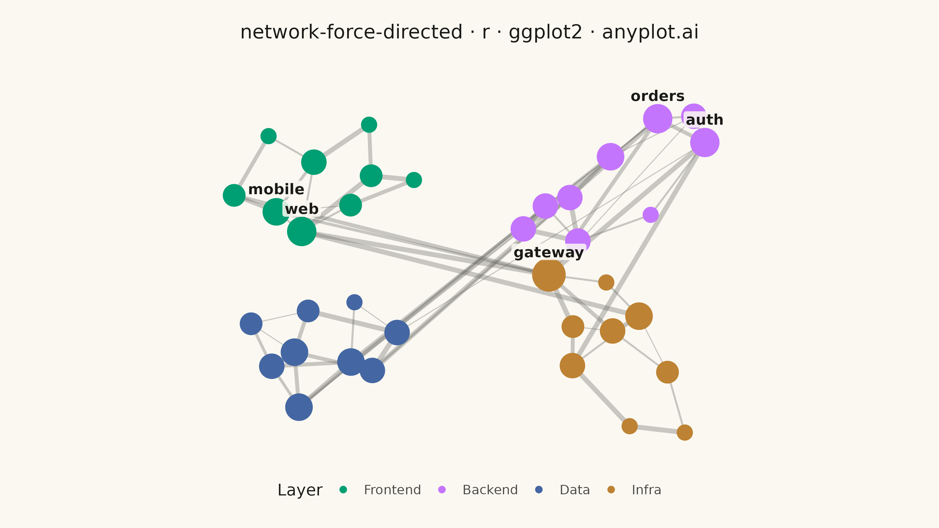
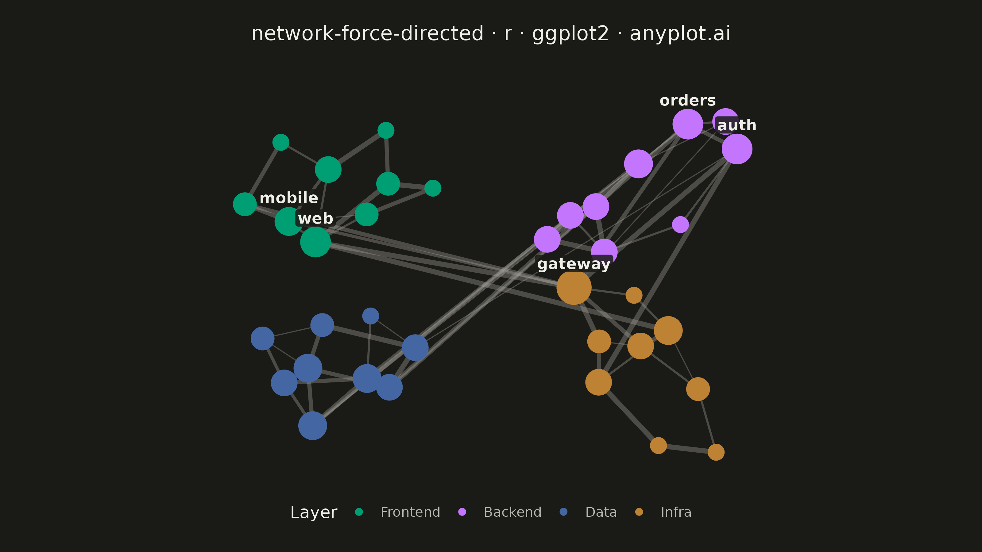
The same plot in 14 other libraries — Python: Altair, Bokeh, lets-plot, Matplotlib, Plotly, plotnine, Pygal, Seaborn; Julia: Makie.jl; JavaScript: Chart.js, D3.js, Apache ECharts, Highcharts, MUI X Charts. Compare all 15 side by side: Force-Directed Graph in Python, R, Julia and JavaScript.
A force-directed graph uses physics simulation to position nodes, where connected nodes attract each other and all nodes repel. This creates organic layouts that naturally reveal community structure, central nodes, and overall network topology without manual positioning. The algorithm balances attractive forces (edges pulling connected nodes together) and repulsive forces (nodes pushing apart) until reaching equilibrium.
#' anyplot.ai
#' network-force-directed: Force-Directed Graph
#' Library: ggplot2 3.5.1 | R 4.4.1
#' Quality: 87/100 | Created: 2026-08-24
library(ggplot2)
library(dplyr)
library(ragg)

set.seed(42)

# --- Theme tokens -----------------------------------------------------------
THEME       <- Sys.getenv("ANYPLOT_THEME", "light")
PAGE_BG     <- if (THEME == "light") "#FAF8F1" else "#1A1A17"
INK         <- if (THEME == "light") "#1A1A17" else "#F0EFE8"
INK_SOFT    <- if (THEME == "light") "#4A4A44" else "#B8B7B0"
INK_MUTED   <- if (THEME == "light") "#6B6A63" else "#A8A79F"
IMPRINT_PALETTE <- c("#009E73", "#C475FD", "#4467A3", "#BD8233",
                     "#AE3030", "#2ABCCD", "#954477", "#99B314")

# --- Data: microservice dependency graph, grouped by architectural layer ---
layers <- list(
  Frontend = c("web", "mobile", "admin", "embed", "portal", "kiosk", "docs", "sdk", "cli"),
  Backend  = c("auth", "users", "orders", "payments", "notify", "search", "catalog", "pricing", "shipping"),
  Data     = c("db-primary", "db-replica", "cache", "queue", "warehouse", "lake", "etl", "backup", "index"),
  Infra    = c("gateway", "lb", "cdn", "dns", "monitor", "logging", "secrets", "ci", "registry")
)

nodes <- tibble(
  id      = unlist(layers, use.names = FALSE),
  cluster = rep(names(layers), times = lengths(layers))
)

# Within-layer edges: a ring plus a handful of random chords per layer
intra_edges <- bind_rows(lapply(layers, function(ids) {
  n <- length(ids)
  ring <- tibble(from = ids, to = ids[c(2:n, 1)])
  chord_i <- sample.int(n, size = round(n * 0.55))
  chords <- tibble(
    from = ids[chord_i],
    to   = ids[sapply(chord_i, function(i) sample(setdiff(seq_len(n), i), 1))]
  )
  bind_rows(ring, chords)
}))

# Cross-layer edges: calls that cross architectural boundaries
bridge_edges <- tibble(
  from = c("web", "mobile", "admin", "gateway", "gateway", "gateway", "auth",
           "orders", "payments", "catalog", "search", "notify", "orders",
           "etl", "warehouse", "ci", "monitor", "secrets", "cdn", "lb"),
  to   = c("gateway", "gateway", "gateway", "auth", "users", "orders", "cache",
           "db-primary", "db-primary", "index", "index", "queue", "queue",
           "warehouse", "lake", "registry", "logging", "auth", "web", "gateway")
)

edges <- bind_rows(intra_edges, bridge_edges) %>%
  mutate(pair_key = ifelse(from < to, paste(from, to), paste(to, from))) %>%
  distinct(pair_key, .keep_all = TRUE) %>%
  filter(from != to) %>%
  select(from, to) %>%
  mutate(weight = sample(1:5, n(), replace = TRUE))

degree <- bind_rows(
  edges %>% count(id = from),
  edges %>% count(id = to)
) %>%
  group_by(id) %>%
  summarise(degree = sum(n), .groups = "drop")

nodes <- nodes %>%
  left_join(degree, by = "id") %>%
  mutate(degree = coalesce(degree, 0))

# --- Force-directed layout (Fruchterman-Reingold) ---------------------------
n_nodes  <- nrow(nodes)
area     <- 4
k_ideal  <- sqrt(area / n_nodes)
pos      <- matrix(runif(n_nodes * 2, -1, 1), ncol = 2)
from_idx <- match(edges$from, nodes$id)
to_idx   <- match(edges$to, nodes$id)
n_iter   <- 400
temp     <- 0.15

for (iter in seq_len(n_iter)) {
  dx   <- outer(pos[, 1], pos[, 1], "-")
  dy   <- outer(pos[, 2], pos[, 2], "-")
  dist <- sqrt(dx^2 + dy^2)
  diag(dist) <- Inf
  repulse <- (k_ideal^2) / dist
  disp    <- cbind(rowSums(repulse * dx / dist), rowSums(repulse * dy / dist))

  edge_dx   <- pos[from_idx, 1] - pos[to_idx, 1]
  edge_dy   <- pos[from_idx, 2] - pos[to_idx, 2]
  edge_dist <- pmax(sqrt(edge_dx^2 + edge_dy^2), 1e-6)
  attract   <- (edge_dist^2) / k_ideal
  attract_x <- (edge_dx / edge_dist) * attract
  attract_y <- (edge_dy / edge_dist) * attract

  for (e in seq_along(from_idx)) {
    disp[from_idx[e], 1] <- disp[from_idx[e], 1] - attract_x[e]
    disp[from_idx[e], 2] <- disp[from_idx[e], 2] - attract_y[e]
    disp[to_idx[e], 1]   <- disp[to_idx[e], 1] + attract_x[e]
    disp[to_idx[e], 2]   <- disp[to_idx[e], 2] + attract_y[e]
  }

  disp_len <- pmax(sqrt(rowSums(disp^2)), 1e-6)
  step     <- pmin(disp_len, temp)
  pos      <- pos + (disp / disp_len) * step
  temp     <- temp * 0.99
}

nodes$x <- pos[, 1]
nodes$y <- pos[, 2]

# Re-center each layer's centroid onto a fixed quadrant anchor (matching the
# wide 16:9 canvas) so the four architectural layers spread across all four
# corners instead of drifting along a single diagonal and leaving the
# opposite corners empty. Intra-layer structure from the FR simulation above
# is preserved; only the whole-cluster offset changes.
anchor_x <- c(Frontend = -1.4, Backend = 1.4, Data = -1.4, Infra = 1.4)
anchor_y <- c(Frontend = 0.8, Backend = 0.8, Data = -0.8, Infra = -0.8)
nodes <- nodes %>%
  group_by(cluster) %>%
  mutate(x = x - mean(x) + anchor_x[cluster[1]], y = y - mean(y) + anchor_y[cluster[1]]) %>%
  ungroup()

edge_positions <- edges %>%
  left_join(nodes %>% select(id, x, y), by = c("from" = "id")) %>%
  left_join(nodes %>% select(id, xend = x, yend = y), by = c("to" = "id"))

hub_nodes <- nodes %>% slice_max(degree, n = 5, with_ties = FALSE)
nodes$cluster <- factor(nodes$cluster, levels = names(layers))

# --- Plot ---------------------------------------------------------------
p <- ggplot() +
  geom_segment(
    data = edge_positions,
    aes(x = x, y = y, xend = xend, yend = yend, linewidth = weight),
    color = INK_MUTED, alpha = 0.35, lineend = "round"
  ) +
  geom_point(
    data = nodes,
    aes(x = x, y = y, color = cluster, size = degree)
  ) +
  geom_label(
    data = hub_nodes,
    aes(x = x, y = y, label = id),
    color = INK, fill = PAGE_BG, alpha = 0.85, label.size = NA,
    size = 3.2, fontface = "bold", nudge_y = 0.22,
    label.padding = unit(0.12, "lines")
  ) +
  scale_color_manual(values = IMPRINT_PALETTE[1:4], name = "Layer") +
  scale_size_continuous(range = c(4, 9), guide = "none") +
  scale_linewidth_continuous(range = c(0.3, 1.4), guide = "none") +
  scale_x_continuous(expand = expansion(mult = 0.1)) +
  scale_y_continuous(expand = expansion(mult = 0.1)) +
  coord_equal() +
  labs(title = "network-force-directed · r · ggplot2 · anyplot.ai") +
  theme_void(base_size = 8) +
  theme(
    plot.background   = element_rect(fill = PAGE_BG, color = PAGE_BG),
    panel.background  = element_rect(fill = PAGE_BG, color = NA),
    plot.title        = element_text(color = INK, size = 12, hjust = 0.5, margin = margin(b = 12)),
    legend.position   = "bottom",
    legend.title      = element_text(color = INK, size = 10),
    legend.text       = element_text(color = INK_SOFT, size = 8),
    legend.background = element_rect(fill = PAGE_BG, color = NA),
    legend.key        = element_rect(fill = PAGE_BG, color = NA),
    plot.margin       = margin(15, 15, 15, 15)
  )

# --- Save ---------------------------------------------------------------
ggsave(
  filename = sprintf("plot-%s.png", THEME),
  plot     = p,
  device   = ragg::agg_png,
  width    = 8,
  height   = 4.5,
  units    = "in",
  dpi      = 400
)
Runnable source as JSON, for any HTTP client: https://api.anyplot.ai/specs/network-force-directed/ggplot2/code. Any spec id and library id listed in llms-full.txt fit the same URL shape; every URL below is complete and callable.
{
  "spec_id": "network-force-directed",
  "language": "r",
  "library": "ggplot2",
  "page": "https://anyplot.ai/network-force-directed/r/ggplot2",
  "hub": "https://anyplot.ai/network-force-directed",
  "code_json": "https://api.anyplot.ai/specs/network-force-directed/ggplot2/code",
  "spec_json": "https://api.anyplot.ai/specs/network-force-directed",
  "render_light_png": "https://storage.googleapis.com/anyplot-images/plots/network-force-directed/r/ggplot2/plot-light.png",
  "render_dark_png": "https://storage.googleapis.com/anyplot-images/plots/network-force-directed/r/ggplot2/plot-dark.png",
  "quality_score": 87.0,
  "license": "MIT",
  "guide": "https://anyplot.ai/llms.txt"
}
Part of Force-Directed Graph on anyplot.ai.