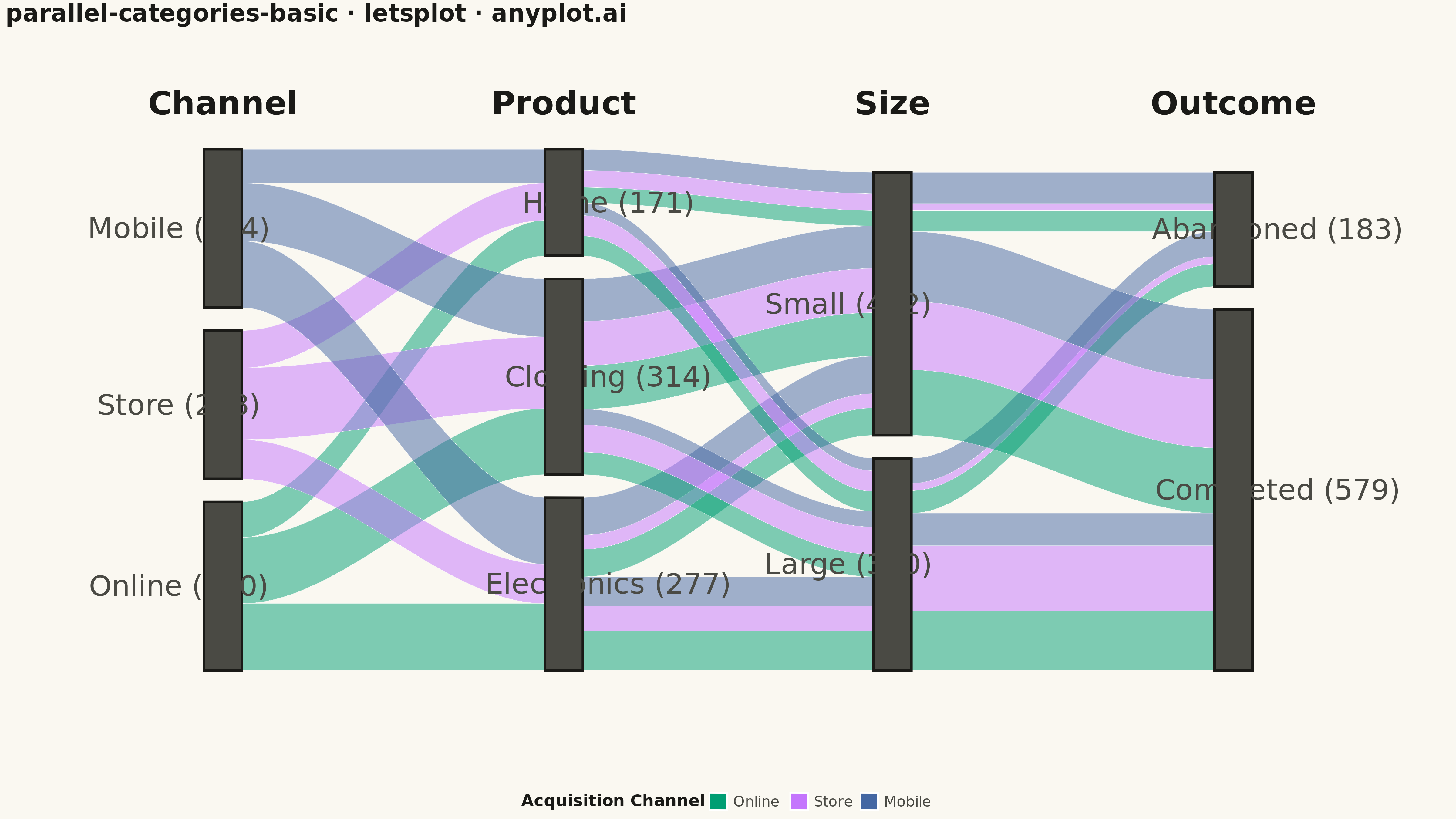
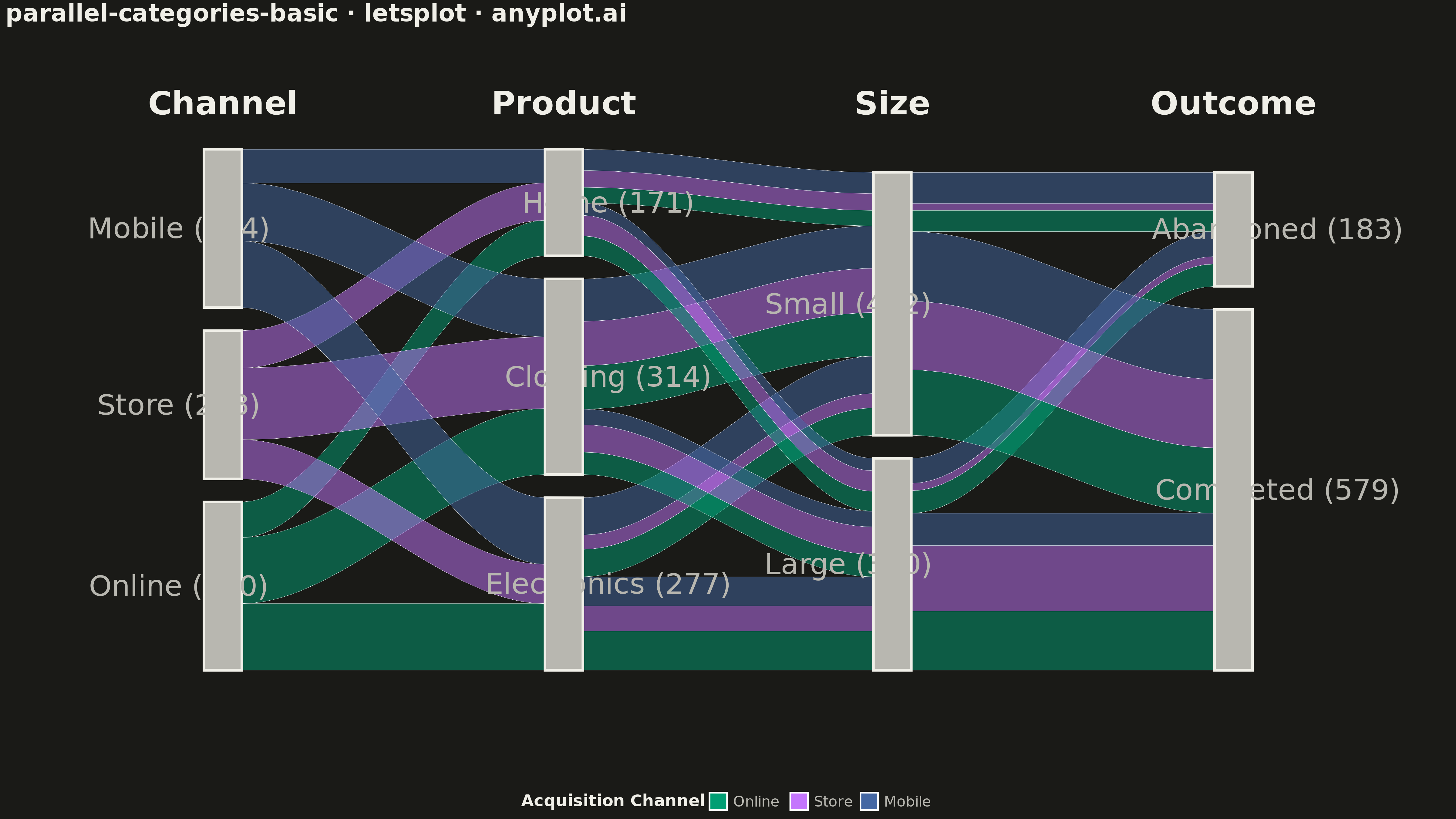
A parallel categories plot visualizes categorical data across multiple dimensions, with vertical axes representing each categorical variable and ribbons connecting categories to show observation flow. Unlike parallel coordinates (which use lines for numeric data), parallel categories use width-proportional ribbons to show counts or frequencies, making it ideal for understanding how categorical values co-occur and flow across multiple classification dimensions.
""" anyplot.ai
parallel-categories-basic: Basic Parallel Categories Plot
Library: letsplot 4.9.0 | Python 3.13.13
Quality: 93/100 | Updated: 2026-05-13
"""

import os

import pandas as pd
from lets_plot import (
    LetsPlot,
    aes,
    element_blank,
    element_rect,
    element_text,
    geom_polygon,
    geom_rect,
    geom_text,
    ggplot,
    ggsize,
    labs,
    scale_fill_manual,
    scale_x_continuous,
    scale_y_continuous,
    theme,
    theme_minimal,
)
from lets_plot.export import ggsave


LetsPlot.setup_html()

# Theme tokens
THEME = os.getenv("ANYPLOT_THEME", "light")
PAGE_BG = "#FAF8F1" if THEME == "light" else "#1A1A17"
ELEVATED_BG = "#FFFDF6" if THEME == "light" else "#242420"
INK = "#1A1A17" if THEME == "light" else "#F0EFE8"
INK_SOFT = "#4A4A44" if THEME == "light" else "#B8B7B0"

# Okabe-Ito palette (first 3 colors for the 3 channels)
IMPRINT = ["#009E73", "#C475FD", "#4467A3"]

# Customer journey data with multiple categorical dimensions
# Dimensions: Channel (acquisition), Product Category, Purchase Size, Outcome
data = [
    # Online channel journeys
    ("Online", "Electronics", "Large", "Completed", 45),
    ("Online", "Electronics", "Small", "Completed", 32),
    ("Online", "Electronics", "Large", "Abandoned", 18),
    ("Online", "Electronics", "Small", "Abandoned", 12),
    ("Online", "Clothing", "Large", "Completed", 28),
    ("Online", "Clothing", "Small", "Completed", 55),
    ("Online", "Clothing", "Large", "Abandoned", 8),
    ("Online", "Clothing", "Small", "Abandoned", 15),
    ("Online", "Home", "Large", "Completed", 22),
    ("Online", "Home", "Small", "Completed", 18),
    ("Online", "Home", "Large", "Abandoned", 10),
    ("Online", "Home", "Small", "Abandoned", 7),
    # Store channel journeys
    ("Store", "Electronics", "Large", "Completed", 35),
    ("Store", "Electronics", "Small", "Completed", 20),
    ("Store", "Electronics", "Large", "Abandoned", 5),
    ("Store", "Electronics", "Small", "Abandoned", 3),
    ("Store", "Clothing", "Large", "Completed", 40),
    ("Store", "Clothing", "Small", "Completed", 65),
    ("Store", "Clothing", "Large", "Abandoned", 4),
    ("Store", "Clothing", "Small", "Abandoned", 6),
    ("Store", "Home", "Large", "Completed", 30),
    ("Store", "Home", "Small", "Completed", 25),
    ("Store", "Home", "Large", "Abandoned", 3),
    ("Store", "Home", "Small", "Abandoned", 2),
    # Mobile channel journeys
    ("Mobile", "Electronics", "Large", "Completed", 25),
    ("Mobile", "Electronics", "Small", "Completed", 42),
    ("Mobile", "Electronics", "Large", "Abandoned", 22),
    ("Mobile", "Electronics", "Small", "Abandoned", 18),
    ("Mobile", "Clothing", "Large", "Completed", 15),
    ("Mobile", "Clothing", "Small", "Completed", 48),
    ("Mobile", "Clothing", "Large", "Abandoned", 10),
    ("Mobile", "Clothing", "Small", "Abandoned", 20),
    ("Mobile", "Home", "Large", "Completed", 12),
    ("Mobile", "Home", "Small", "Completed", 22),
    ("Mobile", "Home", "Large", "Abandoned", 8),
    ("Mobile", "Home", "Small", "Abandoned", 12),
]

# Define dimensions and their categories
dimensions = ["Channel", "Product", "Size", "Outcome"]
categories = {
    "Channel": ["Online", "Store", "Mobile"],
    "Product": ["Electronics", "Clothing", "Home"],
    "Size": ["Large", "Small"],
    "Outcome": ["Completed", "Abandoned"],
}

# Colors for the first dimension (Channel) - using Okabe-Ito palette
channel_colors = {"Online": IMPRINT[0], "Store": IMPRINT[1], "Mobile": IMPRINT[2]}

# Calculate totals for each dimension-category combination
dimension_totals = {dim: {} for dim in dimensions}
for channel, product, size, outcome, count in data:
    dimension_totals["Channel"][channel] = dimension_totals["Channel"].get(channel, 0) + count
    dimension_totals["Product"][product] = dimension_totals["Product"].get(product, 0) + count
    dimension_totals["Size"][size] = dimension_totals["Size"].get(size, 0) + count
    dimension_totals["Outcome"][outcome] = dimension_totals["Outcome"].get(outcome, 0) + count

total_flow = sum(count for _, _, _, _, count in data)

# Layout parameters - increased spacing for better label readability
x_positions = [0.10, 0.37, 0.63, 0.90]
node_width = 0.030
node_gap = 0.035

# Calculate node positions for all dimensions (flat structure)
node_positions = []
for dim_idx in range(len(dimensions)):
    dim = dimensions[dim_idx]
    positions = {}
    y_offset = 0.10
    for cat in categories[dim]:
        height = dimension_totals[dim].get(cat, 0) / total_flow * 0.72
        positions[cat] = {"y0": y_offset, "y1": y_offset + height, "x": x_positions[dim_idx]}
        y_offset += height + node_gap
    node_positions.append(positions)

# Build flow polygons between adjacent dimensions
flow_data = []

# Process each pair of adjacent dimensions
for dim_from_idx in range(len(dimensions) - 1):
    dim_to_idx = dim_from_idx + 1
    dim_from = dimensions[dim_from_idx]
    dim_to = dimensions[dim_to_idx]

    # Aggregate flows between categories
    flow_counts = {}
    for channel, product, size, outcome, count in data:
        values = {"Channel": channel, "Product": product, "Size": size, "Outcome": outcome}
        from_cat = values[dim_from]
        to_cat = values[dim_to]
        source_channel = channel
        key = (from_cat, to_cat, source_channel)
        flow_counts[key] = flow_counts.get(key, 0) + count

    # Track offsets for positioning flows within nodes
    from_offsets = dict.fromkeys(categories[dim_from], 0)
    to_offsets = dict.fromkeys(categories[dim_to], 0)

    from_positions = node_positions[dim_from_idx]
    to_positions = node_positions[dim_to_idx]

    x_left = x_positions[dim_from_idx] + node_width / 2
    x_right = x_positions[dim_to_idx] - node_width / 2

    # Sort flows for consistent ordering
    sorted_flows = sorted(
        flow_counts.items(),
        key=lambda x: (
            categories[dim_from].index(x[0][0]),
            categories[dim_to].index(x[0][1]),
            list(channel_colors.keys()).index(x[0][2]),
        ),
    )

    for (from_cat, to_cat, source_channel), count in sorted_flows:
        flow_height = count / total_flow * 0.72

        src_y0 = from_positions[from_cat]["y0"] + from_offsets[from_cat]
        src_y1 = src_y0 + flow_height
        from_offsets[from_cat] += flow_height

        tgt_y0 = to_positions[to_cat]["y0"] + to_offsets[to_cat]
        tgt_y1 = tgt_y0 + flow_height
        to_offsets[to_cat] += flow_height

        # Create smooth curve polygon with easing
        n_points = 30
        x_vals_top = []
        y_vals_top = []
        x_vals_bottom = []
        y_vals_bottom = []

        for i in range(n_points + 1):
            t = i / n_points
            x = x_left + t * (x_right - x_left)
            ease = t * t * (3 - 2 * t)
            y_top = src_y1 + ease * (tgt_y1 - src_y1)
            y_bottom = src_y0 + ease * (tgt_y0 - src_y0)

            x_vals_top.append(x)
            y_vals_top.append(y_top)
            x_vals_bottom.append(x)
            y_vals_bottom.append(y_bottom)

        # Combine into closed polygon
        x_polygon = x_vals_top + x_vals_bottom[::-1]
        y_polygon = y_vals_top + y_vals_bottom[::-1]

        flow_id = f"d{dim_from_idx}_{from_cat}_{to_cat}_{source_channel}"
        for x, y in zip(x_polygon, y_polygon, strict=False):
            flow_data.append(
                {"x": x, "y": y, "flow_id": flow_id, "channel": source_channel, "from_cat": from_cat, "to_cat": to_cat}
            )

df_flows = pd.DataFrame(flow_data)

# Build node rectangles
node_rects = []
for dim_idx, dim in enumerate(dimensions):
    for cat in categories[dim]:
        pos = node_positions[dim_idx][cat]
        node_rects.append(
            {
                "xmin": pos["x"] - node_width / 2,
                "xmax": pos["x"] + node_width / 2,
                "ymin": pos["y0"],
                "ymax": pos["y1"],
                "category": cat,
                "dimension": dim,
            }
        )

df_nodes = pd.DataFrame(node_rects)

# Build labels
labels = []

# Dimension headers at top
for i, dim in enumerate(dimensions):
    labels.append({"x": x_positions[i], "y": 0.96, "label": dim, "type": "header", "hjust": 0.5})

# Category labels with counts - positioned with more spacing
for dim_idx, dim in enumerate(dimensions):
    for cat in categories[dim]:
        pos = node_positions[dim_idx][cat]
        count = dimension_totals[dim][cat]

        # Position labels on outer sides for first/last dimensions, alternating for middle
        if dim_idx == 0:
            x_label = pos["x"] - node_width / 2 - 0.02
            hjust = 1
        elif dim_idx == len(dimensions) - 1:
            x_label = pos["x"] + node_width / 2 + 0.02
            hjust = 0
        elif dim_idx % 2 == 0:
            x_label = pos["x"] - node_width / 2 - 0.02
            hjust = 1
        else:
            x_label = pos["x"] + node_width / 2 + 0.02
            hjust = 0

        labels.append(
            {
                "x": x_label,
                "y": (pos["y0"] + pos["y1"]) / 2,
                "label": f"{cat} ({count})",
                "type": "category",
                "hjust": hjust,
            }
        )

df_labels = pd.DataFrame(labels)

# Create the plot
plot = (
    ggplot()
    + geom_polygon(
        aes(x="x", y="y", group="flow_id", fill="channel"), data=df_flows, alpha=0.5, color="white", size=0.08
    )
    + geom_rect(
        aes(xmin="xmin", xmax="xmax", ymin="ymin", ymax="ymax"), data=df_nodes, fill=INK_SOFT, color=INK, size=1.2
    )
    + geom_text(
        aes(x="x", y="y", label="label"),
        data=df_labels[df_labels["type"] == "header"],
        size=18,
        hjust=0.5,
        fontface="bold",
        color=INK,
    )
    + geom_text(
        aes(x="x", y="y", label="label"), data=df_labels[df_labels["type"] == "category"], size=16, color=INK_SOFT
    )
    + scale_fill_manual(
        values={
            "Online": channel_colors["Online"],
            "Store": channel_colors["Store"],
            "Mobile": channel_colors["Mobile"],
        },
        name="Acquisition Channel",
    )
    + labs(title="parallel-categories-basic · letsplot · anyplot.ai")
    + theme_minimal()
    + theme(
        plot_background=element_rect(fill=PAGE_BG, color=PAGE_BG),
        panel_background=element_rect(fill=PAGE_BG, color=PAGE_BG),
        plot_title=element_text(size=26, face="bold", color=INK),
        axis_title=element_blank(),
        axis_text=element_blank(),
        axis_ticks=element_blank(),
        panel_grid=element_blank(),
        legend_text=element_text(size=16, color=INK_SOFT),
        legend_title=element_text(size=18, face="bold", color=INK),
        legend_position="bottom",
        legend_background=element_blank(),
    )
    + scale_x_continuous(limits=[-0.02, 1.02])
    + scale_y_continuous(limits=[-0.02, 1.02])
    + ggsize(1600, 900)
)

# Save as PNG (scale 3x for 4800 × 2700 px) and HTML
ggsave(plot, f"plot-{THEME}.png", path=".", scale=3)
ggsave(plot, f"plot-{THEME}.html", path=".")
Runnable source as JSON, for any HTTP client: https://api.anyplot.ai/specs/parallel-categories-basic/letsplot/code. Any spec id and library id listed in llms-full.txt fit the same URL shape; every URL below is complete and callable.
{
  "spec_id": "parallel-categories-basic",
  "language": "python",
  "library": "letsplot",
  "page": "https://anyplot.ai/parallel-categories-basic/python/letsplot",
  "hub": "https://anyplot.ai/parallel-categories-basic",
  "code_json": "https://api.anyplot.ai/specs/parallel-categories-basic/letsplot/code",
  "spec_json": "https://api.anyplot.ai/specs/parallel-categories-basic",
  "render_light_png": "https://storage.googleapis.com/anyplot-images/plots/parallel-categories-basic/python/letsplot/plot-light.png",
  "render_dark_png": "https://storage.googleapis.com/anyplot-images/plots/parallel-categories-basic/python/letsplot/plot-dark.png",
  "interactive_light_html": "https://storage.googleapis.com/anyplot-images/plots/parallel-categories-basic/python/letsplot/plot-light.html",
  "interactive_dark_html": "https://storage.googleapis.com/anyplot-images/plots/parallel-categories-basic/python/letsplot/plot-dark.html",
  "quality_score": 93.0,
  "license": "MIT",
  "guide": "https://anyplot.ai/llms.txt"
}
Part of Basic Parallel Categories Plot on anyplot.ai.