The same plot in 14 other libraries — Python: Altair, Bokeh, lets-plot, Matplotlib, Plotly, plotnine, Pygal, Seaborn; Julia: Makie.jl; JavaScript: Chart.js, D3.js, Apache ECharts, Highcharts, MUI X Charts. Compare all 15 side by side: Basic Parallel Categories Plot in Python, R, Julia and JavaScript.
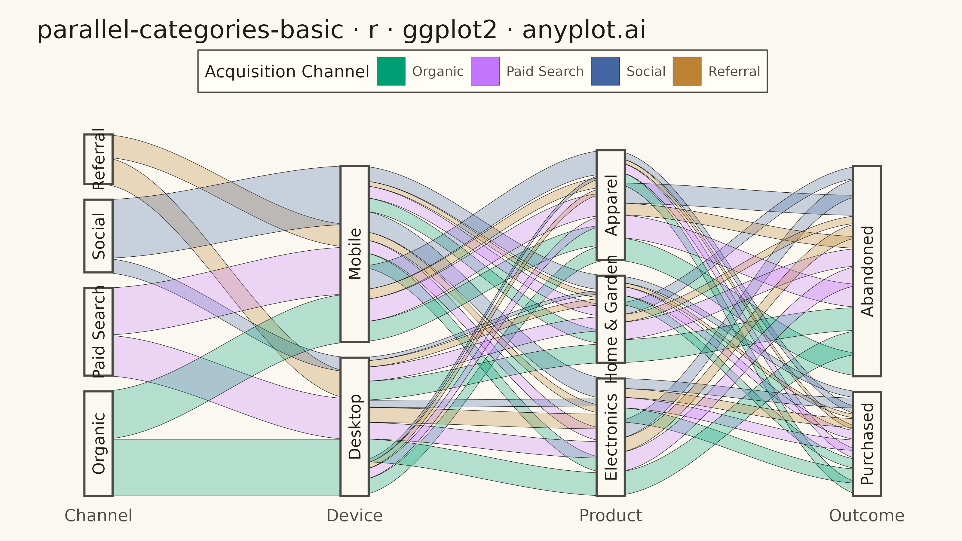
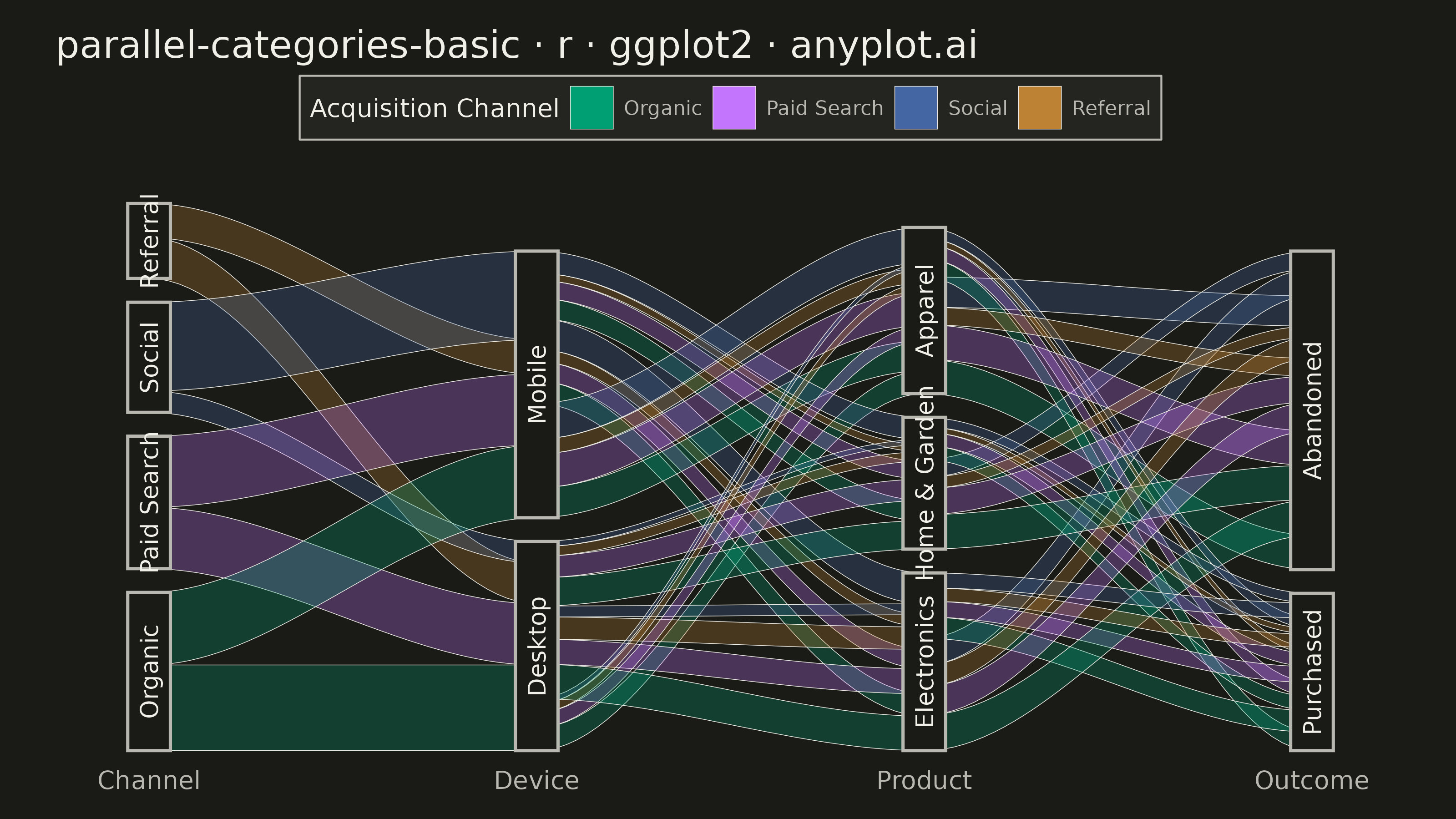
A parallel categories plot visualizes categorical data across multiple dimensions, with vertical axes representing each categorical variable and ribbons connecting categories to show observation flow. Unlike parallel coordinates (which use lines for numeric data), parallel categories use width-proportional ribbons to show counts or frequencies, making it ideal for understanding how categorical values co-occur and flow across multiple classification dimensions.
#' anyplot.ai
#' parallel-categories-basic: Basic Parallel Categories Plot
#' Library: ggplot2 3.5.1 | R 4.4.1
#' Quality: 81/100 | Created: 2026-09-05

library(ggplot2)
library(dplyr)
library(ragg)

set.seed(42)

# --- Theme tokens -------------------------------------------------------
THEME       <- Sys.getenv("ANYPLOT_THEME", "light")
PAGE_BG     <- if (THEME == "light") "#FAF8F1" else "#1A1A17"
ELEVATED_BG <- if (THEME == "light") "#FFFDF6" else "#242420"
INK         <- if (THEME == "light") "#1A1A17" else "#F0EFE8"
INK_SOFT    <- if (THEME == "light") "#4A4A44" else "#B8B7B0"

# Imprint palette (see prompts/default-style-guide.md "Categorical Palette")
IMPRINT_PALETTE <- c("#009E73", "#C475FD", "#4467A3", "#BD8233",
                     "#AE3030", "#2ABCCD", "#954477", "#99B314")

NODE_WIDTH <- 0.055

# --- Data: customer journey across 4 categorical dimensions -------------
# ggplot2 has no native parallel-categories geom (ggalluvial is not installed
# in this environment) — bands below are built from first principles with
# stacked node ranges and a smoothstep interpolation, using only geom_ribbon
# and geom_rect, both native ggplot2 geoms. Colored by the first dimension
# (acquisition channel), so a customer's ribbon keeps its origin hue as it
# flows through every subsequent stage.
channel_levels <- c("Organic", "Paid Search", "Social", "Referral")
device_levels  <- c("Desktop", "Mobile")
product_levels <- c("Electronics", "Apparel", "Home & Garden")
outcome_levels <- c("Purchased", "Abandoned")

channel_probs <- c(Organic = 0.32, "Paid Search" = 0.28, Social = 0.24, Referral = 0.16)

device_probs_by_channel <- list(
  Organic       = c(Desktop = 0.55, Mobile = 0.45),
  "Paid Search" = c(Desktop = 0.42, Mobile = 0.58),
  Social        = c(Desktop = 0.22, Mobile = 0.78),
  Referral      = c(Desktop = 0.60, Mobile = 0.40)
)

product_probs_by_device <- list(
  Desktop = c(Electronics = 0.45, Apparel = 0.25, "Home & Garden" = 0.30),
  Mobile  = c(Electronics = 0.30, Apparel = 0.45, "Home & Garden" = 0.25)
)

outcome_probs_by_product <- list(
  Electronics     = c(Purchased = 0.38, Abandoned = 0.62),
  Apparel         = c(Purchased = 0.30, Abandoned = 0.70),
  "Home & Garden" = c(Purchased = 0.35, Abandoned = 0.65)
)

n_customers <- 2000
channel <- sample(names(channel_probs), n_customers, replace = TRUE, prob = channel_probs)
device  <- vapply(channel, function(ch) {
  probs <- device_probs_by_channel[[ch]]
  sample(names(probs), 1, prob = probs)
}, character(1))
product <- vapply(device, function(d) {
  probs <- product_probs_by_device[[d]]
  sample(names(probs), 1, prob = probs)
}, character(1))
outcome <- vapply(product, function(p) {
  probs <- outcome_probs_by_product[[p]]
  sample(names(probs), 1, prob = probs)
}, character(1))

# --- Crossing-minimization: order each downstream stage by the weighted
# barycenter of its predecessor's node positions (forward Sugiyama sweep),
# instead of fixed definition order, so fewer ribbons cross between hops.
barycenter_order <- function(from_vec, to_vec, prev_order) {
  prev_pos <- setNames(seq_along(prev_order), prev_order)
  agg <- as.data.frame(table(from = from_vec, to = to_vec), stringsAsFactors = FALSE)
  categories <- unique(agg$to)
  bary <- vapply(categories, function(cat) {
    rows <- agg[agg$to == cat, ]
    sum(prev_pos[rows$from] * rows$Freq) / sum(rows$Freq)
  }, numeric(1))
  categories[order(bary)]
}

device_order  <- barycenter_order(channel, device, channel_levels)
product_order <- barycenter_order(device, product, device_order)
outcome_order <- barycenter_order(product, outcome, product_order)

df <- tibble::tibble(
  channel = factor(channel, levels = channel_levels),
  device  = factor(device,  levels = device_order),
  product = factor(product, levels = product_order),
  outcome = factor(outcome, levels = outcome_order)
)

# --- Node totals & stacked y-ranges per stage (crossing-minimized order) ----
# GAP is deliberately generous (5% of n, vs. a typical 2-3%) to open up
# breathing room between stacked nodes at each stage, since the Device->Product
# and Product->Outcome hops carry many crossing ribbons.
GAP <- n_customers * 0.05

node_totals_for <- function(values, stage_x) {
  tibble::tibble(category = values) %>%
    count(category, name = "total") %>%
    mutate(category = factor(category, levels = levels(values))) %>%
    arrange(category) %>%
    mutate(
      ymax     = cumsum(total) + GAP * (row_number() - 1),
      ymin     = ymax - total,
      stage    = stage_x,
      category = as.character(category)
    )
}

node_channel <- node_totals_for(df$channel, 1)
node_device  <- node_totals_for(df$device,  2)
node_product <- node_totals_for(df$product, 3)
node_outcome <- node_totals_for(df$outcome, 4)
node_all <- bind_rows(node_channel, node_device, node_product, node_outcome)

# --- Aggregated flows between adjacent stages, origin = channel ---------
edges_channel_device  <- df %>%
  count(channel, device, name = "value") %>%
  transmute(origin = as.character(channel), from_cat = as.character(channel),
            to_cat = as.character(device), value)

edges_device_product <- df %>%
  count(channel, device, product, name = "value") %>%
  transmute(origin = as.character(channel), from_cat = as.character(device),
            to_cat = as.character(product), value)

edges_product_outcome <- df %>%
  count(channel, product, outcome, name = "value") %>%
  transmute(origin = as.character(channel), from_cat = as.character(product),
            to_cat = as.character(outcome), value)

# --- Smooth bands via smoothstep interpolation ---------------------------
build_hop_bands <- function(edges, stage_from, stage_to, node_from, node_to, n_smooth = 40) {
  edges <- edges %>%
    group_by(from_cat) %>%
    arrange(to_cat, origin, .by_group = TRUE) %>%
    mutate(y1_out = cumsum(value), y0_out = y1_out - value) %>%
    ungroup() %>%
    left_join(node_from %>% transmute(from_cat = category, node_ymin_from = ymin), by = "from_cat") %>%
    mutate(y0_from = node_ymin_from + y0_out, y1_from = node_ymin_from + y1_out)

  edges <- edges %>%
    group_by(to_cat) %>%
    arrange(origin, from_cat, .by_group = TRUE) %>%
    mutate(y1_in = cumsum(value), y0_in = y1_in - value) %>%
    ungroup() %>%
    left_join(node_to %>% transmute(to_cat = category, node_ymin_to = ymin), by = "to_cat") %>%
    mutate(y0_to = node_ymin_to + y0_in, y1_to = node_ymin_to + y1_in) %>%
    mutate(edge_id = row_number())

  t <- seq(0, 1, length.out = n_smooth)
  w <- t ^ 2 * (3 - 2 * t)  # smoothstep S-curve

  edges %>%
    rowwise() %>%
    reframe(
      edge_id = edge_id,
      origin  = origin,
      value   = value,
      x       = stage_from + t * (stage_to - stage_from),
      ymin    = y0_from + w * (y0_to - y0_from),
      ymax    = y1_from + w * (y1_to - y1_from)
    )
}

# Largest flows are drawn first (so they sit behind), thinner flows drawn last
# (on top) -- this keeps small paths from getting visually buried under the
# bulk of the crossing traffic in the dense middle hops.
bands <- bind_rows(
  build_hop_bands(edges_channel_device,  1, 2, node_channel, node_device)  %>% mutate(hop = "h1"),
  build_hop_bands(edges_device_product,  2, 3, node_device,  node_product) %>% mutate(hop = "h2"),
  build_hop_bands(edges_product_outcome, 3, 4, node_product, node_outcome) %>% mutate(hop = "h3")
) %>%
  mutate(
    group_id = paste(hop, edge_id, sep = "_"),
    origin   = factor(origin, levels = channel_levels)
  ) %>%
  arrange(desc(value))

# --- Plot ------------------------------------------------------------------
p <- ggplot() +
  geom_ribbon(
    data = bands,
    aes(x = x, ymin = ymin, ymax = ymax, group = group_id, fill = origin),
    color = INK, linewidth = 0.12, alpha = 0.28
  ) +
  geom_rect(
    data = node_all,
    aes(xmin = stage - NODE_WIDTH, xmax = stage + NODE_WIDTH, ymin = ymin, ymax = ymax),
    fill = PAGE_BG, color = INK_SOFT, linewidth = 0.6
  ) +
  geom_text(
    data = node_all,
    aes(x = stage, y = (ymin + ymax) / 2, label = category),
    angle = 90, size = 3.4, color = INK
  ) +
  scale_fill_manual(
    values = setNames(IMPRINT_PALETTE[seq_along(channel_levels)], channel_levels),
    name   = "Acquisition Channel"
  ) +
  scale_x_continuous(
    breaks = 1:4, labels = c("Channel", "Device", "Product", "Outcome"),
    expand = expansion(mult = c(0.06, 0.06))
  ) +
  scale_y_continuous(expand = expansion(mult = c(0.02, 0.08))) +
  guides(fill = guide_legend(override.aes = list(alpha = 1))) +
  labs(
    title = "parallel-categories-basic · r · ggplot2 · anyplot.ai",
    x = NULL, y = NULL
  ) +
  theme_minimal(base_size = 8) +
  theme(
    plot.background   = element_rect(fill = PAGE_BG, color = PAGE_BG),
    panel.background  = element_rect(fill = PAGE_BG, color = NA),
    panel.grid        = element_blank(),
    axis.title        = element_blank(),
    axis.text.y       = element_blank(),
    axis.ticks        = element_blank(),
    axis.text.x       = element_text(color = INK_SOFT, size = 10),
    plot.title        = element_text(color = INK, size = 15),
    legend.position    = "top",
    legend.background = element_rect(fill = ELEVATED_BG, color = INK_SOFT),
    legend.text       = element_text(color = INK_SOFT, size = 8),
    legend.title      = element_text(color = INK, size = 10),
    plot.margin       = margin(12, 20, 10, 20)
  )

# --- Save --------------------------------------------------------------------
ggsave(
  filename = sprintf("plot-%s.png", THEME),
  plot     = p,
  device   = ragg::agg_png,
  width    = 8,
  height   = 4.5,
  units    = "in",
  dpi      = 400
)
Runnable source as JSON, for any HTTP client: https://api.anyplot.ai/specs/parallel-categories-basic/ggplot2/code. Any spec id and library id listed in llms-full.txt fit the same URL shape; every URL below is complete and callable.
{
  "spec_id": "parallel-categories-basic",
  "language": "r",
  "library": "ggplot2",
  "page": "https://anyplot.ai/parallel-categories-basic/r/ggplot2",
  "hub": "https://anyplot.ai/parallel-categories-basic",
  "code_json": "https://api.anyplot.ai/specs/parallel-categories-basic/ggplot2/code",
  "spec_json": "https://api.anyplot.ai/specs/parallel-categories-basic",
  "render_light_png": "https://storage.googleapis.com/anyplot-images/plots/parallel-categories-basic/r/ggplot2/plot-light.png",
  "render_dark_png": "https://storage.googleapis.com/anyplot-images/plots/parallel-categories-basic/r/ggplot2/plot-dark.png",
  "quality_score": 81.0,
  "license": "MIT",
  "guide": "https://anyplot.ai/llms.txt"
}
Part of Basic Parallel Categories Plot on anyplot.ai.