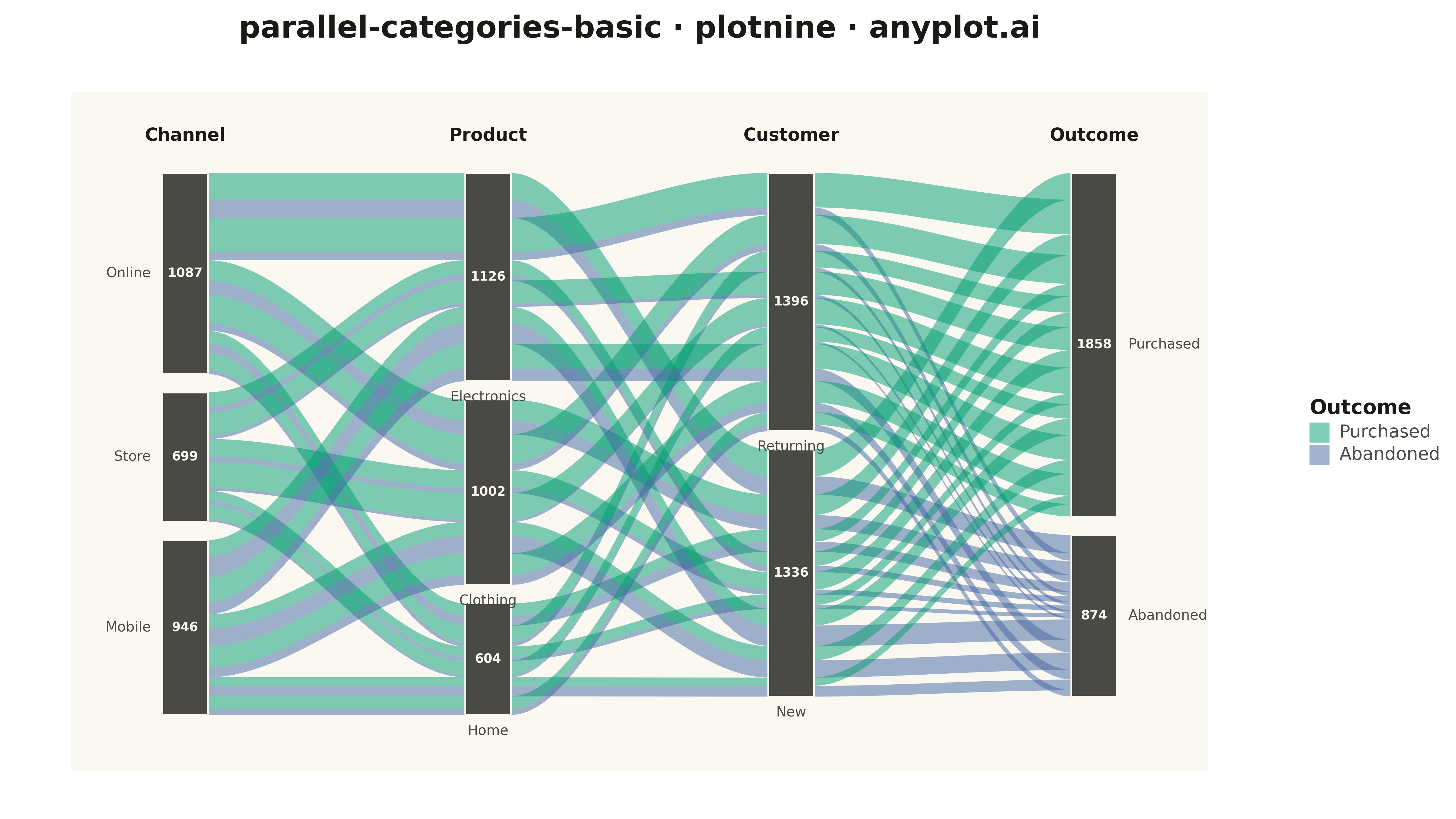
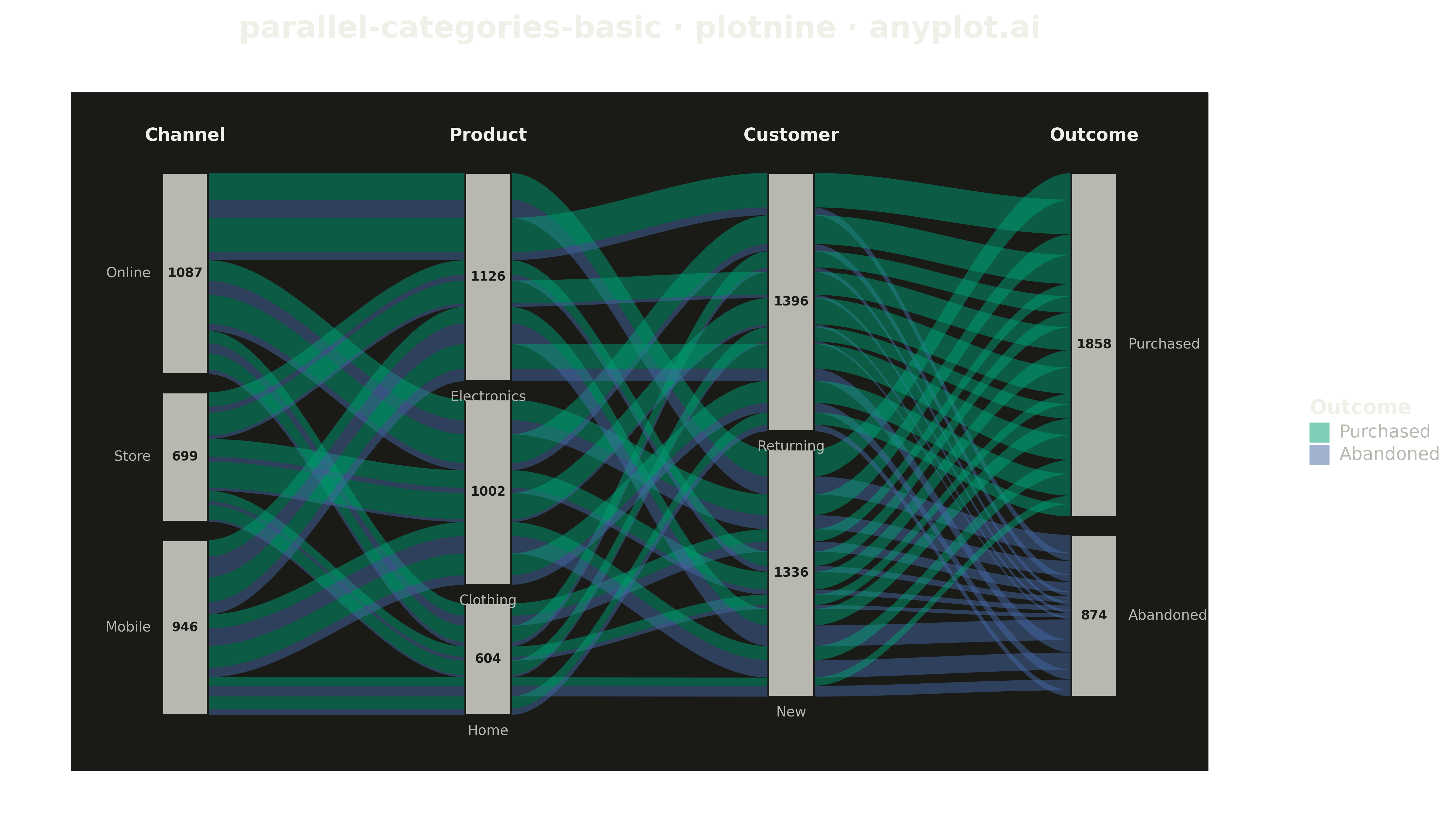
A parallel categories plot visualizes categorical data across multiple dimensions, with vertical axes representing each categorical variable and ribbons connecting categories to show observation flow. Unlike parallel coordinates (which use lines for numeric data), parallel categories use width-proportional ribbons to show counts or frequencies, making it ideal for understanding how categorical values co-occur and flow across multiple classification dimensions.
""" anyplot.ai
parallel-categories-basic: Basic Parallel Categories Plot
Library: plotnine 0.15.4 | Python 3.13.13
Quality: 84/100 | Updated: 2026-05-13
"""

import os
import sys


# Prevent current directory from shadowing the plotnine package
sys.path = [p for p in sys.path if not p.endswith("implementations") and not p.endswith("python")]

import numpy as np
import pandas as pd
from plotnine import (
    aes,
    annotate,
    element_blank,
    element_text,
    geom_polygon,
    geom_rect,
    geom_text,
    ggplot,
    labs,
    scale_fill_manual,
    theme,
    theme_minimal,
)


# Theme tokens
THEME = os.getenv("ANYPLOT_THEME", "light")
PAGE_BG = "#FAF8F1" if THEME == "light" else "#1A1A17"
ELEVATED_BG = "#FFFDF6" if THEME == "light" else "#242420"
INK = "#1A1A17" if THEME == "light" else "#F0EFE8"
INK_SOFT = "#4A4A44" if THEME == "light" else "#B8B7B0"

# Okabe-Ito palette for categorical data
IMPRINT = [
    "#009E73",  # Brand green - first series
    "#C475FD",  # Vermillion
    "#4467A3",  # Blue
    "#BD8233",  # Reddish purple
    "#AE3030",  # Orange
    "#2ABCCD",  # Sky blue
    "#954477",  # Yellow
]

# Data - Customer journey data with multiple categorical dimensions
np.random.seed(42)

# Define category combinations and realistic counts
path_data = [
    # Channel -> Product Category -> Customer Type -> Outcome
    ("Online", "Electronics", "New", "Purchased", 145),
    ("Online", "Electronics", "New", "Abandoned", 98),
    ("Online", "Electronics", "Returning", "Purchased", 187),
    ("Online", "Electronics", "Returning", "Abandoned", 42),
    ("Online", "Clothing", "New", "Purchased", 112),
    ("Online", "Clothing", "New", "Abandoned", 76),
    ("Online", "Clothing", "Returning", "Purchased", 156),
    ("Online", "Clothing", "Returning", "Abandoned", 38),
    ("Online", "Home", "New", "Purchased", 67),
    ("Online", "Home", "New", "Abandoned", 54),
    ("Online", "Home", "Returning", "Purchased", 89),
    ("Online", "Home", "Returning", "Abandoned", 23),
    ("Store", "Electronics", "New", "Purchased", 78),
    ("Store", "Electronics", "New", "Abandoned", 32),
    ("Store", "Electronics", "Returning", "Purchased", 124),
    ("Store", "Electronics", "Returning", "Abandoned", 18),
    ("Store", "Clothing", "New", "Purchased", 95),
    ("Store", "Clothing", "New", "Abandoned", 28),
    ("Store", "Clothing", "Returning", "Purchased", 142),
    ("Store", "Clothing", "Returning", "Abandoned", 15),
    ("Store", "Home", "New", "Purchased", 56),
    ("Store", "Home", "New", "Abandoned", 21),
    ("Store", "Home", "Returning", "Purchased", 78),
    ("Store", "Home", "Returning", "Abandoned", 12),
    ("Mobile", "Electronics", "New", "Purchased", 89),
    ("Mobile", "Electronics", "New", "Abandoned", 112),
    ("Mobile", "Electronics", "Returning", "Purchased", 134),
    ("Mobile", "Electronics", "Returning", "Abandoned", 67),
    ("Mobile", "Clothing", "New", "Purchased", 76),
    ("Mobile", "Clothing", "New", "Abandoned", 94),
    ("Mobile", "Clothing", "Returning", "Purchased", 118),
    ("Mobile", "Clothing", "Returning", "Abandoned", 52),
    ("Mobile", "Home", "New", "Purchased", 45),
    ("Mobile", "Home", "New", "Abandoned", 58),
    ("Mobile", "Home", "Returning", "Purchased", 67),
    ("Mobile", "Home", "Returning", "Abandoned", 34),
]

path_counts = pd.DataFrame(path_data, columns=["channel", "product", "customer_type", "outcome", "count"])

# Define dimensions and their category orders
dimensions = [
    {"name": "channel", "label": "Channel", "categories": ["Online", "Store", "Mobile"]},
    {"name": "product", "label": "Product", "categories": ["Electronics", "Clothing", "Home"]},
    {"name": "customer_type", "label": "Customer", "categories": ["Returning", "New"]},
    {"name": "outcome", "label": "Outcome", "categories": ["Purchased", "Abandoned"]},
]

# Color by outcome - using Okabe-Ito palette
outcome_colors = {
    "Purchased": IMPRINT[0],  # Brand green
    "Abandoned": IMPRINT[2],  # Blue
}

# Layout parameters
n_dims = len(dimensions)
x_positions = np.linspace(0.1, 0.9, n_dims)
node_width = 0.04
node_gap = 0.03
total_height = 0.82
y_start = 0.92

# Calculate node positions for each dimension
node_positions = {}
for dim_idx, dim in enumerate(dimensions):
    x_pos = x_positions[dim_idx]
    categories = dim["categories"]
    col_name = dim["name"]

    # Calculate totals for this dimension
    totals = path_counts.groupby(col_name)["count"].sum()
    grand_total = totals.sum()
    current_y = y_start

    for cat in categories:
        count = totals.get(cat, 0)
        height = (count / grand_total) * total_height if grand_total > 0 else 0

        node_positions[(dim_idx, cat)] = {
            "x": x_pos,
            "y_top": current_y,
            "y_bottom": current_y - height,
            "height": height,
            "count": count,
            "flow_offset_out": 0,
            "flow_offset_in": 0,
        }
        current_y = current_y - height - node_gap

# Build node rectangles dataframe
node_data = []
for (dim_idx, cat), pos in node_positions.items():
    node_data.append(
        {
            "dim_idx": dim_idx,
            "category": cat,
            "xmin": pos["x"] - node_width / 2,
            "xmax": pos["x"] + node_width / 2,
            "ymin": pos["y_bottom"],
            "ymax": pos["y_top"],
            "label_y": (pos["y_top"] + pos["y_bottom"]) / 2,
            "count": pos["count"],
            "display_label": str(cat),
            "fill_color": INK_SOFT,
        }
    )
nodes_df = pd.DataFrame(node_data)

# Build flow polygons between adjacent dimensions
flow_polygons = []
flow_id_counter = 0

for _, path_row in path_counts.iterrows():
    path_values = [path_row["channel"], path_row["product"], path_row["customer_type"], path_row["outcome"]]
    count = path_row["count"]
    outcome = path_row["outcome"]

    # Draw flows between each adjacent pair of dimensions
    for dim_idx in range(n_dims - 1):
        from_cat = path_values[dim_idx]
        to_cat = path_values[dim_idx + 1]

        src_pos = node_positions[(dim_idx, from_cat)]
        tgt_pos = node_positions[(dim_idx + 1, to_cat)]

        # Calculate flow height proportional to count
        src_total = sum(path_counts[path_counts[dimensions[dim_idx]["name"]] == from_cat]["count"])
        flow_height_src = (count / src_total) * src_pos["height"] if src_total > 0 else 0

        tgt_total = sum(path_counts[path_counts[dimensions[dim_idx + 1]["name"]] == to_cat]["count"])
        flow_height_tgt = (count / tgt_total) * tgt_pos["height"] if tgt_total > 0 else 0

        # Source connection point (right side of node)
        src_y_top = src_pos["y_top"] - src_pos["flow_offset_out"]
        src_y_bottom = src_y_top - flow_height_src
        src_pos["flow_offset_out"] += flow_height_src

        # Target connection point (left side of node)
        tgt_y_top = tgt_pos["y_top"] - tgt_pos["flow_offset_in"]
        tgt_y_bottom = tgt_y_top - flow_height_tgt
        tgt_pos["flow_offset_in"] += flow_height_tgt

        # Create curved flow polygon using cubic interpolation
        flow_x_left = x_positions[dim_idx] + node_width / 2
        flow_x_right = x_positions[dim_idx + 1] - node_width / 2
        n_points = 30

        t_param = np.linspace(0, 1, n_points)
        # Smooth cubic easing for natural flow appearance
        x_top = flow_x_left + (flow_x_right - flow_x_left) * t_param
        y_top = src_y_top + (tgt_y_top - src_y_top) * (3 * t_param**2 - 2 * t_param**3)

        x_bottom = flow_x_right + (flow_x_left - flow_x_right) * t_param
        y_bottom = tgt_y_bottom + (src_y_bottom - tgt_y_bottom) * (3 * t_param**2 - 2 * t_param**3)

        # Combine into polygon
        x_polygon = np.concatenate([x_top, x_bottom])
        y_polygon = np.concatenate([y_top, y_bottom])

        flow_id = f"flow_{flow_id_counter}"
        flow_id_counter += 1

        for i in range(len(x_polygon)):
            flow_polygons.append({"x": x_polygon[i], "y": y_polygon[i], "flow_id": flow_id, "outcome": outcome})

flows_df = pd.DataFrame(flow_polygons)

# Create background rectangle data
bg_rect = pd.DataFrame({"xmin": [0], "xmax": [1], "ymin": [-0.05], "ymax": [1.05]})

# Create the plot
plot = (
    ggplot()
    # Background rectangle
    + geom_rect(bg_rect, aes(xmin="xmin", xmax="xmax", ymin="ymin", ymax="ymax"), fill=PAGE_BG, color=PAGE_BG)
    # Flow polygons with transparency - colored by outcome
    + geom_polygon(flows_df, aes(x="x", y="y", group="flow_id", fill="outcome"), alpha=0.5)
    # Node rectangles
    + geom_rect(
        nodes_df, aes(xmin="xmin", xmax="xmax", ymin="ymin", ymax="ymax"), fill=INK_SOFT, color=PAGE_BG, size=0.8
    )
    # Count labels on nodes
    + geom_text(
        nodes_df[nodes_df["count"] >= 20],
        aes(x=(nodes_df["xmin"] + nodes_df["xmax"]) / 2, y="label_y", label="count"),
        ha="center",
        va="center",
        size=10,
        color=PAGE_BG,
        fontweight="bold",
    )
    + scale_fill_manual(values=outcome_colors, name="Outcome", breaks=["Purchased", "Abandoned"])
    + labs(title="parallel-categories-basic · plotnine · anyplot.ai", x="", y="")
    + theme_minimal()
    + theme(
        figure_size=(16, 9),
        plot_background=element_blank(),
        panel_background=element_blank(),
        plot_title=element_text(size=24, ha="center", weight="bold", color=INK),
        axis_text=element_blank(),
        axis_ticks=element_blank(),
        panel_grid=element_blank(),
        legend_background=element_blank(),
        legend_title=element_text(size=16, weight="bold", color=INK),
        legend_text=element_text(size=14, color=INK_SOFT),
        legend_position="right",
    )
)

# Add dimension labels at top
for dim_idx, dim in enumerate(dimensions):
    plot = plot + annotate(
        "text", x=x_positions[dim_idx], y=0.98, label=dim["label"], size=14, color=INK, fontweight="bold", ha="center"
    )

# Add category labels beside each node
for (dim_idx, cat), pos in node_positions.items():
    label = str(cat)
    label_y = (pos["y_top"] + pos["y_bottom"]) / 2

    # For first dimension, place label on left side of node
    if dim_idx == 0:
        plot = plot + annotate(
            "text",
            x=x_positions[dim_idx] - node_width / 2 - 0.01,
            y=label_y,
            label=label,
            size=11,
            color=INK_SOFT,
            ha="right",
            va="center",
        )
    # For last dimension, place label on right side of node
    elif dim_idx == n_dims - 1:
        plot = plot + annotate(
            "text",
            x=x_positions[dim_idx] + node_width / 2 + 0.01,
            y=label_y,
            label=label,
            size=11,
            color=INK_SOFT,
            ha="left",
            va="center",
        )
    # For middle dimensions, place label below the node
    else:
        plot = plot + annotate(
            "text",
            x=x_positions[dim_idx],
            y=pos["y_bottom"] - 0.015,
            label=label,
            size=11,
            color=INK_SOFT,
            ha="center",
            va="top",
        )

plot.save(f"plot-{THEME}.png", dpi=300, verbose=False)
Runnable source as JSON, for any HTTP client: https://api.anyplot.ai/specs/parallel-categories-basic/plotnine/code. Any spec id and library id listed in llms-full.txt fit the same URL shape; every URL below is complete and callable.
{
  "spec_id": "parallel-categories-basic",
  "language": "python",
  "library": "plotnine",
  "page": "https://anyplot.ai/parallel-categories-basic/python/plotnine",
  "hub": "https://anyplot.ai/parallel-categories-basic",
  "code_json": "https://api.anyplot.ai/specs/parallel-categories-basic/plotnine/code",
  "spec_json": "https://api.anyplot.ai/specs/parallel-categories-basic",
  "render_light_png": "https://storage.googleapis.com/anyplot-images/plots/parallel-categories-basic/python/plotnine/plot-light.png",
  "render_dark_png": "https://storage.googleapis.com/anyplot-images/plots/parallel-categories-basic/python/plotnine/plot-dark.png",
  "quality_score": 84.0,
  "license": "MIT",
  "guide": "https://anyplot.ai/llms.txt"
}
Part of Basic Parallel Categories Plot on anyplot.ai.