The same plot in 14 other libraries — Python: Altair, Bokeh, lets-plot, Matplotlib, Plotly, plotnine, Pygal, Seaborn; Julia: Makie.jl; JavaScript: Chart.js, D3.js, Apache ECharts, Highcharts, MUI X Charts. Compare all 15 side by side: Basic Polar Chart in Python, R, Julia and JavaScript.
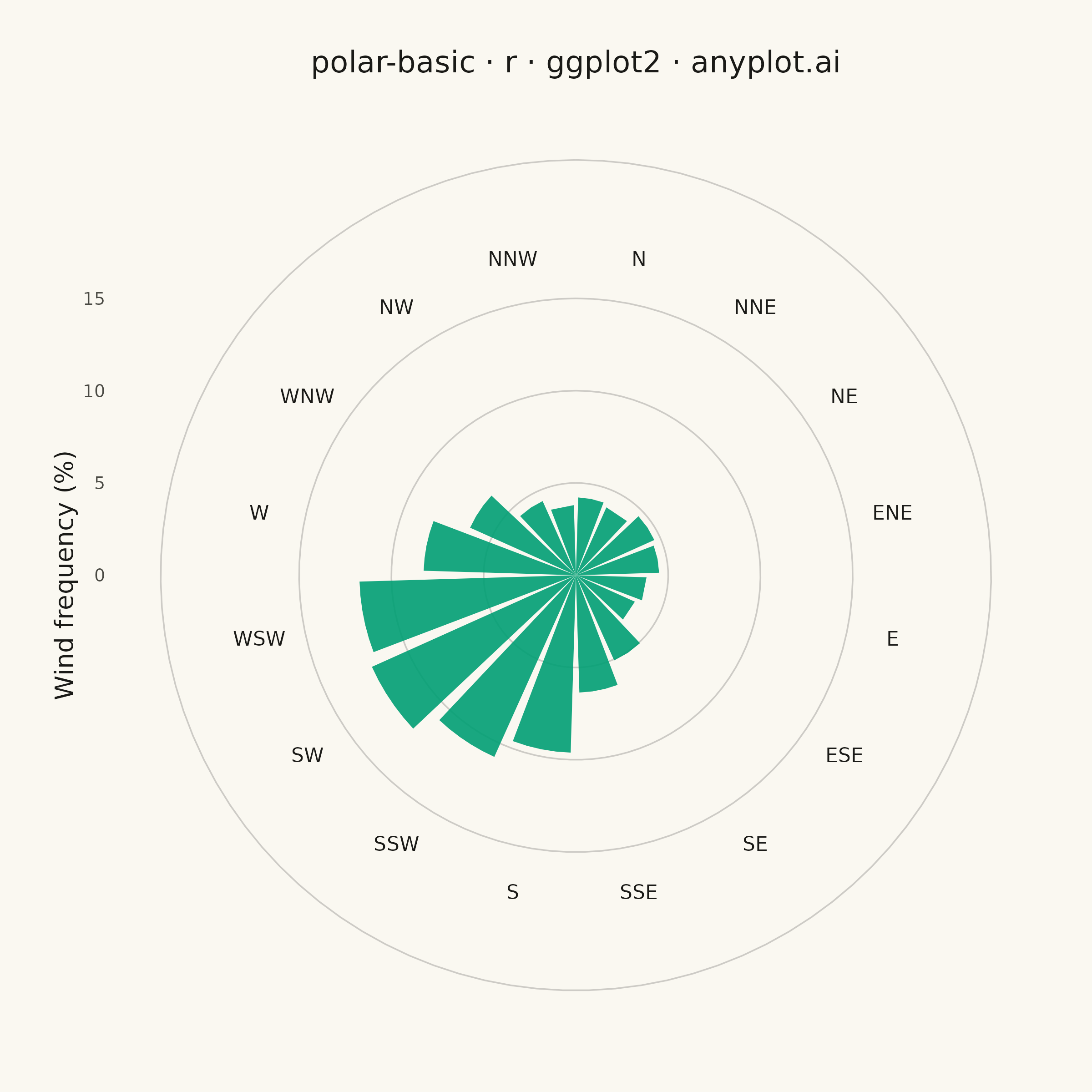
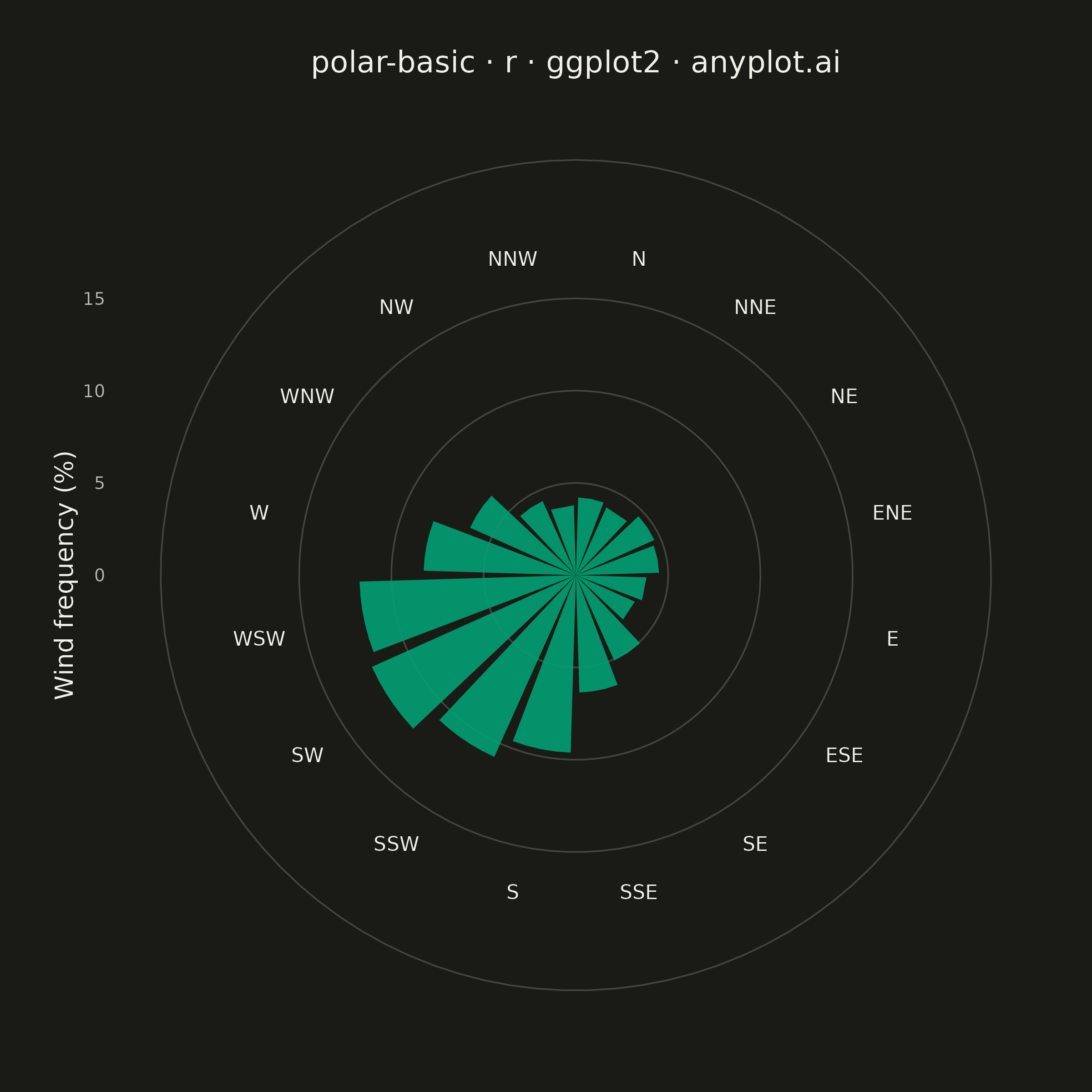
A polar chart displays data points on a circular coordinate system where position is determined by angle (theta) and distance from center (radius). This visualization is ideal for cyclical patterns, directional data, or any dataset where angular relationships are meaningful. It reveals periodic trends and directional distributions that would be obscured in Cartesian coordinates.
#' anyplot.ai
#' polar-basic: Basic Polar Chart
#' Library: ggplot2 3.5.1 | R 4.4.1
#' Quality: 89/100 | Updated: 2026-07-25

library(ggplot2)
library(ragg)
library(scales)

set.seed(42)

# --- Theme tokens -------------------------------------------------------
THEME <- Sys.getenv("ANYPLOT_THEME", "light")
PAGE_BG <- if (THEME == "light") "#FAF8F1" else "#1A1A17"
INK <- if (THEME == "light") "#1A1A17" else "#F0EFE8"
INK_SOFT <- if (THEME == "light") "#4A4A44" else "#B8B7B0"
IMPRINT_PALETTE <- c(
    "#009E73", "#C475FD", "#4467A3", "#BD8233",
    "#AE3030", "#2ABCCD", "#954477", "#99B314"
)
BRAND <- IMPRINT_PALETTE[1]

# --- Data -----------------------------------------------------------------
# Wind direction frequency at a coastal weather station, 16-point compass.
compass_directions <- c(
    "N", "NNE", "NE", "ENE", "E", "ESE", "SE", "SSE",
    "S", "SSW", "SW", "WSW", "W", "WNW", "NW", "NNW"
)
n_directions <- length(compass_directions)
direction_index <- seq_len(n_directions)
prevailing_index <- 11 # SW - prevailing onshore wind for this station
land_breeze_index <- 3 # NE - opposite direction, secondary nighttime land-breeze peak

angular_distance <- function(center) {
    pmin(abs(direction_index - center), n_directions - abs(direction_index - center))
}

# Dominant onshore SW wind plus a smaller offshore NE land-breeze counter-peak.
prevailing_bump <- exp(-0.5 * (angular_distance(prevailing_index) / 2.6)^2)
land_breeze_bump <- 0.35 * exp(-0.5 * (angular_distance(land_breeze_index) / 2.0)^2)
base_frequency <- prevailing_bump + land_breeze_bump + 0.05

# A frequency distribution across all 16 directions must sum to 100%, so
# normalize before adding measurement noise.
base_frequency <- base_frequency / sum(base_frequency) * 100
wind_frequency <- pmax(base_frequency + rnorm(n_directions, 0, 0.4), 0.3)

wind_rose <- tibble::tibble(
    direction = factor(compass_directions, levels = compass_directions),
    frequency = wind_frequency
)

# coord_polar always draws its outer boundary circle at the axis maximum,
# exactly where the default theta-axis labels sit (a ggplot2 rendering
# quirk, not a theme setting) - so compass labels are placed manually at a
# radius comfortably inside that boundary instead of via axis.text.x.
grid_max <- ceiling(max(wind_frequency) / 5) * 5
label_radius <- grid_max + 2.5
boundary_limit <- grid_max + 5
compass_labels <- tibble::tibble(
    direction = factor(compass_directions, levels = compass_directions),
    label_radius = label_radius
)

# --- Plot -------------------------------------------------------------------
p <- ggplot(wind_rose, aes(x = direction, y = frequency)) +
    geom_col(fill = BRAND, width = 0.85, alpha = 0.9) +
    geom_text(
        data = compass_labels,
        aes(x = direction, y = label_radius, label = direction),
        inherit.aes = FALSE, color = INK, size = 2.8
    ) +
    coord_polar(theta = "x") +
    scale_y_continuous(
        limits = c(0, boundary_limit),
        breaks = seq(0, grid_max, by = 5),
        expand = c(0, 0)
    ) +
    labs(
        title = "polar-basic · r · ggplot2 · anyplot.ai",
        x = NULL,
        y = "Wind frequency (%)"
    ) +
    theme_minimal(base_size = 8) +
    theme(
        plot.background = element_rect(fill = PAGE_BG, color = PAGE_BG),
        panel.background = element_rect(fill = PAGE_BG, color = NA),
        panel.grid.major.x = element_blank(),
        panel.grid.major.y = element_line(color = scales::alpha(INK, 0.2), linewidth = 0.3),
        panel.grid.minor = element_blank(),
        axis.title.x = element_blank(),
        axis.title.y = element_text(color = INK, size = 10),
        axis.text.x = element_blank(),
        axis.text.y = element_text(color = INK_SOFT, size = 7),
        axis.ticks = element_blank(),
        plot.title = element_text(color = INK, size = 12, hjust = 0.5, margin = margin(b = 14)),
        plot.margin = margin(20, 20, 20, 20)
    )

# --- Save -------------------------------------------------------------------
ggsave(
    filename = sprintf("plot-%s.png", THEME),
    plot = p,
    device = ragg::agg_png,
    width = 6,
    height = 6,
    units = "in",
    dpi = 400
)
Runnable source as JSON, for any HTTP client: https://api.anyplot.ai/specs/polar-basic/ggplot2/code. Any spec id and library id listed in llms-full.txt fit the same URL shape; every URL below is complete and callable.
{
  "spec_id": "polar-basic",
  "language": "r",
  "library": "ggplot2",
  "page": "https://anyplot.ai/polar-basic/r/ggplot2",
  "hub": "https://anyplot.ai/polar-basic",
  "code_json": "https://api.anyplot.ai/specs/polar-basic/ggplot2/code",
  "spec_json": "https://api.anyplot.ai/specs/polar-basic",
  "render_light_png": "https://storage.googleapis.com/anyplot-images/plots/polar-basic/r/ggplot2/plot-light.png",
  "render_dark_png": "https://storage.googleapis.com/anyplot-images/plots/polar-basic/r/ggplot2/plot-dark.png",
  "quality_score": 89.0,
  "license": "MIT",
  "guide": "https://anyplot.ai/llms.txt"
}
Part of Basic Polar Chart on anyplot.ai.