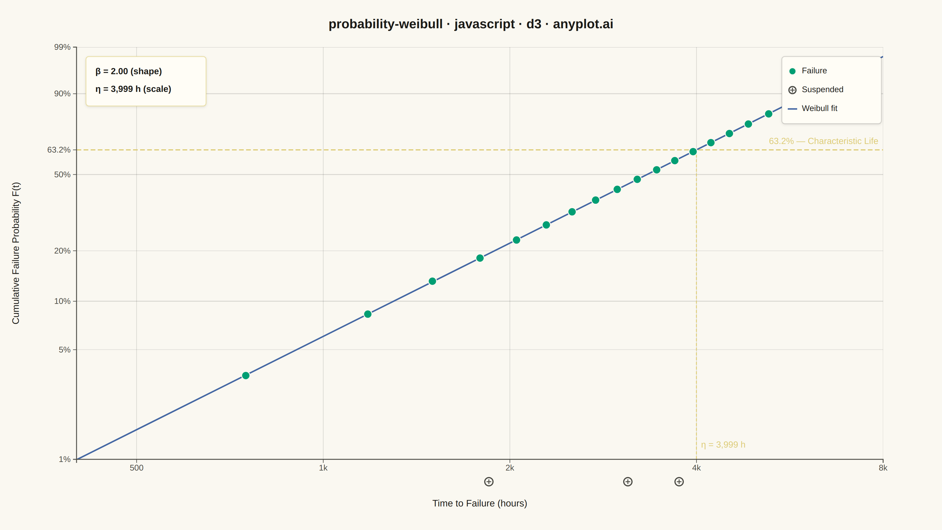
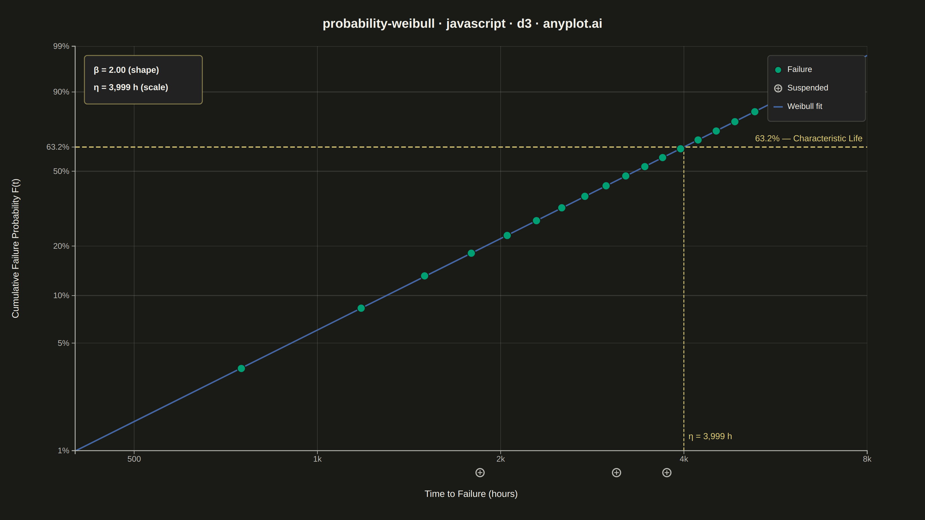
The same plot in 14 other libraries — JavaScript: Chart.js, Apache ECharts, Highcharts, MUI X Charts; Python: Altair, Bokeh, lets-plot, Matplotlib, Plotly, plotnine, Pygal, Seaborn; R: ggplot2; Julia: Makie.jl. Compare all 15 side by side: Weibull Probability Plot for Reliability Analysis in Python, R, Julia and JavaScript.
A Weibull probability plot displays failure or lifetime data on Weibull probability paper (logarithmic x-axis for time/cycles, linearized Weibull CDF on y-axis) with a fitted straight line. It is the standard tool in reliability engineering for estimating Weibull distribution parameters (shape and scale), assessing whether data follow a Weibull distribution, and extrapolating failure probabilities. The slope of the fitted line gives the shape parameter (beta), while the characteristic life (eta) is read at the 63.2% failure probability crossing.
// anyplot.ai
// probability-weibull: Weibull Probability Plot for Reliability Analysis
// Library: d3 7.9.0 | JavaScript 22.22.3
// Quality: 91/100 | Created: 2026-06-07

const t = window.ANYPLOT_TOKENS;
const { width, height } = window.ANYPLOT_SIZE;

const margin = { top: 80, right: 100, bottom: 120, left: 130 };
const iw = width - margin.left - margin.right;
const ih = height - margin.top - margin.bottom;

// Turbine blade fatigue-life data: 17 failures + 3 right-censored suspensions
// Times approximate Weibull(β≈2, η≈4000 h) — sorted by time
const rawData = [
  { time: 750,  failed: true  },
  { time: 1180, failed: true  },
  { time: 1500, failed: true  },
  { time: 1790, failed: true  },
  { time: 1850, failed: false },
  { time: 2050, failed: true  },
  { time: 2290, failed: true  },
  { time: 2520, failed: true  },
  { time: 2750, failed: true  },
  { time: 2980, failed: true  },
  { time: 3100, failed: false },
  { time: 3210, failed: true  },
  { time: 3450, failed: true  },
  { time: 3690, failed: true  },
  { time: 3750, failed: false },
  { time: 3950, failed: true  },
  { time: 4220, failed: true  },
  { time: 4520, failed: true  },
  { time: 4850, failed: true  },
  { time: 5230, failed: true  },
];

const n = rawData.length;
const weibullY = (F) => Math.log(-Math.log(1 - F));

// Bernard's median rank: (i − 0.3) / (n + 0.4)
let failRank = 0;
const plotData = rawData.map((d) => {
  if (d.failed) {
    failRank++;
    const F = (failRank - 0.3) / (n + 0.4);
    return { time: d.time, failed: true, F, yw: weibullY(F) };
  }
  return { time: d.time, failed: false, F: null, yw: null };
});

const failures = plotData.filter((d) => d.failed);
const censored = plotData.filter((d) => !d.failed);

// OLS regression in Weibull coordinates: yw = β·ln(t) + b
const lnT = (d) => Math.log(d.time);
const nF  = failures.length;
const sx  = d3.sum(failures, lnT);
const sy  = d3.sum(failures, (d) => d.yw);
const sxy = d3.sum(failures, (d) => lnT(d) * d.yw);
const sxx = d3.sum(failures, (d) => lnT(d) * lnT(d));
const beta       = (nF * sxy - sx * sy) / (nF * sxx - sx * sx);
const bIntercept = (sy - beta * sx) / nF;
const eta        = Math.round(Math.exp(-bIntercept / beta));

// Probability axis ticks — major (heavier) and minor (lighter) for Weibull paper texture
const majorProbs = [0.01, 0.1, 0.5, 0.9, 0.99];
const minorProbs = [0.05, 0.2];
const allProbs   = [0.01, 0.05, 0.1, 0.2, 0.5, 0.632, 0.9, 0.99];
const yMin = weibullY(0.01);
const yMax = weibullY(0.99);

// SVG + defs (clip path + subtle drop-shadow filter for info boxes)
const svg = d3.select("#container").append("svg").attr("width", width).attr("height", height);
const defs = svg.append("defs");
defs.append("clipPath").attr("id", "plot-clip")
  .append("rect").attr("width", iw).attr("height", ih);
const shadowFilter = defs.append("filter")
  .attr("id", "box-shadow").attr("x", "-20%").attr("y", "-20%").attr("width", "140%").attr("height", "140%");
shadowFilter.append("feDropShadow")
  .attr("dx", 0).attr("dy", 1.5).attr("stdDeviation", 2.5).attr("flood-color", "rgba(0,0,0,0.10)");

const g     = svg.append("g").attr("transform", `translate(${margin.left},${margin.top})`);
const plotG = g.append("g").attr("clip-path", "url(#plot-clip)");

// Scales
const x = d3.scaleLog().domain([400, 8000]).range([0, iw]);
const y = d3.scaleLinear().domain([yMin, yMax]).range([ih, 0]);

// Horizontal grid — major ticks heavier (1.5px), minor lighter (0.75px) to mimic Weibull paper
majorProbs.forEach((F) => {
  plotG.append("line")
    .attr("x1", 0).attr("x2", iw)
    .attr("y1", y(weibullY(F))).attr("y2", y(weibullY(F)))
    .attr("stroke", t.grid).attr("stroke-width", 1.5);
});
minorProbs.forEach((F) => {
  plotG.append("line")
    .attr("x1", 0).attr("x2", iw)
    .attr("y1", y(weibullY(F))).attr("y2", y(weibullY(F)))
    .attr("stroke", t.grid).attr("stroke-width", 0.75);
});
// Vertical grid at log-decade ticks
[500, 1000, 2000, 4000, 8000].forEach((v) => {
  plotG.append("line")
    .attr("x1", x(v)).attr("x2", x(v)).attr("y1", 0).attr("y2", ih)
    .attr("stroke", t.grid).attr("stroke-width", 1);
});

// 63.2% characteristic life reference line (amber dashed)
const y632 = y(weibullY(0.632));
plotG.append("line")
  .attr("x1", 0).attr("x2", iw).attr("y1", y632).attr("y2", y632)
  .attr("stroke", t.amber).attr("stroke-width", 2).attr("stroke-dasharray", "8 4");

if (eta >= 400 && eta <= 8000) {
  plotG.append("line")
    .attr("x1", x(eta)).attr("x2", x(eta)).attr("y1", y632).attr("y2", ih)
    .attr("stroke", t.amber).attr("stroke-width", 1.5).attr("stroke-dasharray", "5 3");
}

// Fitted Weibull line using d3.line() generator
const lineGen = d3.line().x((d) => x(d.tx)).y((d) => y(d.yw));
const fitData = [400, 8000].map((tx) => ({ tx, yw: beta * Math.log(tx) + bIntercept }));
plotG.append("path")
  .datum(fitData).attr("d", lineGen)
  .attr("stroke", t.palette[2]).attr("stroke-width", 2.5).attr("fill", "none");

// Failure points — filled green circles
plotG.selectAll(".fail")
  .data(failures).join("circle").attr("class", "fail")
  .attr("cx", (d) => x(d.time)).attr("cy", (d) => y(d.yw))
  .attr("r", 7)
  .attr("fill", t.palette[0]).attr("stroke", t.pageBg).attr("stroke-width", 1.5);

// Y-axis: idiomatic d3.axisLeft with Weibull probability tick formatting
const yAxis = d3.axisLeft(y)
  .tickValues(allProbs.map(weibullY))
  .tickFormat((yw) => {
    const F = 1 - Math.exp(-Math.exp(yw));
    if (Math.abs(F - 0.632) < 0.002) return "63.2%";
    return `${Math.round(F * 100)}%`;
  })
  .tickSize(6);
const yAxisG = g.append("g").call(yAxis);
yAxisG.selectAll(".tick text").attr("fill", t.inkSoft).style("font-size", "14px").attr("x", -10);
yAxisG.selectAll(".tick line").attr("stroke", t.inkSoft);
yAxisG.select(".domain").attr("stroke", t.inkSoft).attr("stroke-width", 1.5);

// X-axis: idiomatic d3.axisBottom with custom log tick values
const xAxis = d3.axisBottom(x)
  .tickValues([500, 1000, 2000, 4000, 8000])
  .tickFormat((v) => v >= 1000 ? `${v / 1000}k` : `${v}`)
  .tickSize(6);
const xAxisG = g.append("g").attr("transform", `translate(0,${ih})`).call(xAxis);
xAxisG.selectAll(".tick text").attr("fill", t.inkSoft).style("font-size", "14px");
xAxisG.selectAll(".tick line").attr("stroke", t.inkSoft);
xAxisG.select(".domain").attr("stroke", t.inkSoft).attr("stroke-width", 1.5);

// Censored suspensions: hollow + crosshair markers below x-axis
censored.forEach((d) => {
  const cx = x(d.time);
  const cy = ih + 38;
  g.append("circle").attr("cx", cx).attr("cy", cy).attr("r", 7)
    .attr("fill", "none").attr("stroke", t.inkSoft).attr("stroke-width", 2);
  g.append("line").attr("x1", cx - 4).attr("x2", cx + 4).attr("y1", cy).attr("y2", cy)
    .attr("stroke", t.inkSoft).attr("stroke-width", 1.5);
  g.append("line").attr("x1", cx).attr("x2", cx).attr("y1", cy - 4).attr("y2", cy + 4)
    .attr("stroke", t.inkSoft).attr("stroke-width", 1.5);
});

// Amber annotations at 15px for clear readability
g.append("text").attr("x", iw - 8).attr("y", y632 - 10)
  .attr("text-anchor", "end").attr("fill", t.amber)
  .style("font-size", "15px").style("font-weight", "500")
  .text("63.2% — Characteristic Life");

if (eta >= 400 && eta <= 8000) {
  g.append("text").attr("x", x(eta) + 8).attr("y", ih - 20)
    .attr("fill", t.amber).style("font-size", "15px").style("font-weight", "500")
    .text(`η = ${eta.toLocaleString()} h`);
}

// Parameter box — generous padding, amber accent border, drop shadow
const pX = 16, pY = 16;
g.append("rect").attr("x", pX).attr("y", pY).attr("width", 204).attr("height", 84)
  .attr("fill", t.elevatedBg).attr("rx", 5)
  .attr("stroke", t.amber).attr("stroke-width", 1.5).attr("stroke-opacity", 0.55)
  .attr("filter", "url(#box-shadow)");
g.append("text").attr("x", pX + 16).attr("y", pY + 30)
  .attr("fill", t.ink).style("font-size", "15px").style("font-weight", "600")
  .text(`β = ${beta.toFixed(2)}  (shape)`);
g.append("text").attr("x", pX + 16).attr("y", pY + 60)
  .attr("fill", t.ink).style("font-size", "15px").style("font-weight", "600")
  .text(`η = ${eta.toLocaleString()} h  (scale)`);

// Legend — generous padding, neutral border, drop shadow
const lx = iw - 172, ly = 16;
g.append("rect").attr("x", lx).attr("y", ly).attr("width", 169).attr("height", 114)
  .attr("fill", t.elevatedBg).attr("rx", 5)
  .attr("stroke", t.grid).attr("stroke-width", 1.5)
  .attr("filter", "url(#box-shadow)");
// Failure row
g.append("circle").attr("cx", lx + 18).attr("cy", ly + 25).attr("r", 6)
  .attr("fill", t.palette[0]).attr("stroke", t.pageBg).attr("stroke-width", 1.5);
g.append("text").attr("x", lx + 34).attr("y", ly + 25)
  .attr("dominant-baseline", "middle").attr("fill", t.ink).style("font-size", "14px").text("Failure");
// Suspended row
g.append("circle").attr("cx", lx + 18).attr("cy", ly + 57).attr("r", 6)
  .attr("fill", "none").attr("stroke", t.inkSoft).attr("stroke-width", 2);
g.append("line").attr("x1", lx + 14).attr("x2", lx + 22).attr("y1", ly + 57).attr("y2", ly + 57)
  .attr("stroke", t.inkSoft).attr("stroke-width", 1.5);
g.append("line").attr("x1", lx + 18).attr("x2", lx + 18).attr("y1", ly + 53).attr("y2", ly + 61)
  .attr("stroke", t.inkSoft).attr("stroke-width", 1.5);
g.append("text").attr("x", lx + 34).attr("y", ly + 57)
  .attr("dominant-baseline", "middle").attr("fill", t.ink).style("font-size", "14px").text("Suspended");
// Weibull fit row
g.append("line").attr("x1", lx + 10).attr("x2", lx + 26).attr("y1", ly + 89).attr("y2", ly + 89)
  .attr("stroke", t.palette[2]).attr("stroke-width", 2.5);
g.append("text").attr("x", lx + 34).attr("y", ly + 89)
  .attr("dominant-baseline", "middle").attr("fill", t.ink).style("font-size", "14px").text("Weibull fit");

// Axis labels
g.append("text").attr("x", iw / 2).attr("y", ih + 80)
  .attr("text-anchor", "middle").attr("fill", t.ink)
  .style("font-size", "16px").style("font-weight", "500")
  .text("Time to Failure (hours)");
svg.append("text")
  .attr("transform", `translate(32,${margin.top + ih / 2}) rotate(-90)`)
  .attr("text-anchor", "middle").attr("fill", t.ink)
  .style("font-size", "16px").style("font-weight", "500")
  .text("Cumulative Failure Probability F(t)");

// Title
svg.append("text").attr("x", width / 2).attr("y", 48)
  .attr("text-anchor", "middle").attr("fill", t.ink)
  .style("font-size", "22px").style("font-weight", "600")
  .text("probability-weibull · javascript · d3 · anyplot.ai");
Runnable source as JSON, for any HTTP client: https://api.anyplot.ai/specs/probability-weibull/d3/code. Any spec id and library id listed in llms-full.txt fit the same URL shape; every URL below is complete and callable.
{
  "spec_id": "probability-weibull",
  "language": "javascript",
  "library": "d3",
  "page": "https://anyplot.ai/probability-weibull/javascript/d3",
  "hub": "https://anyplot.ai/probability-weibull",
  "code_json": "https://api.anyplot.ai/specs/probability-weibull/d3/code",
  "spec_json": "https://api.anyplot.ai/specs/probability-weibull",
  "render_light_png": "https://storage.googleapis.com/anyplot-images/plots/probability-weibull/javascript/d3/plot-light.png",
  "render_dark_png": "https://storage.googleapis.com/anyplot-images/plots/probability-weibull/javascript/d3/plot-dark.png",
  "interactive_light_html": "https://storage.googleapis.com/anyplot-images/plots/probability-weibull/javascript/d3/plot-light.html",
  "interactive_dark_html": "https://storage.googleapis.com/anyplot-images/plots/probability-weibull/javascript/d3/plot-dark.html",
  "quality_score": 91.0,
  "license": "MIT",
  "guide": "https://anyplot.ai/llms.txt"
}
Part of Weibull Probability Plot for Reliability Analysis on anyplot.ai.