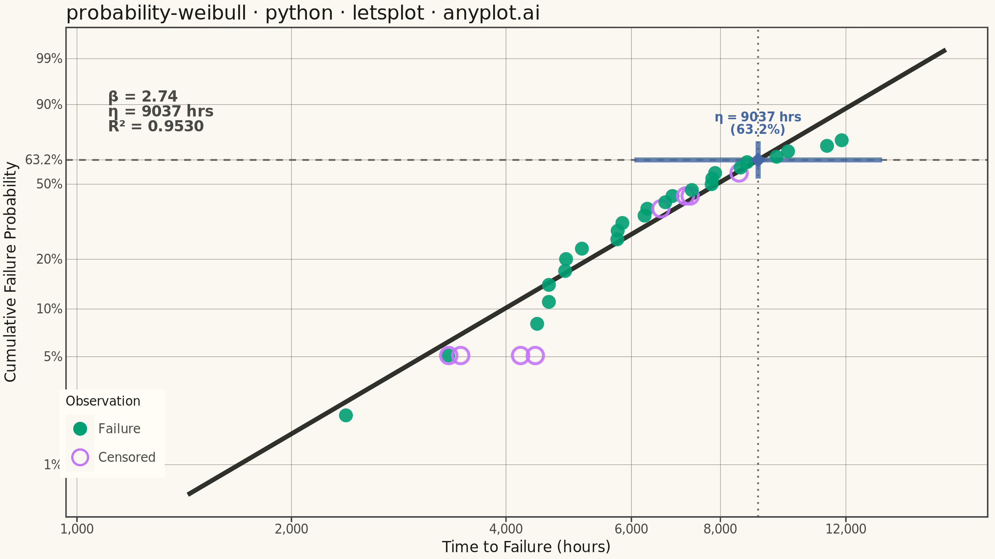
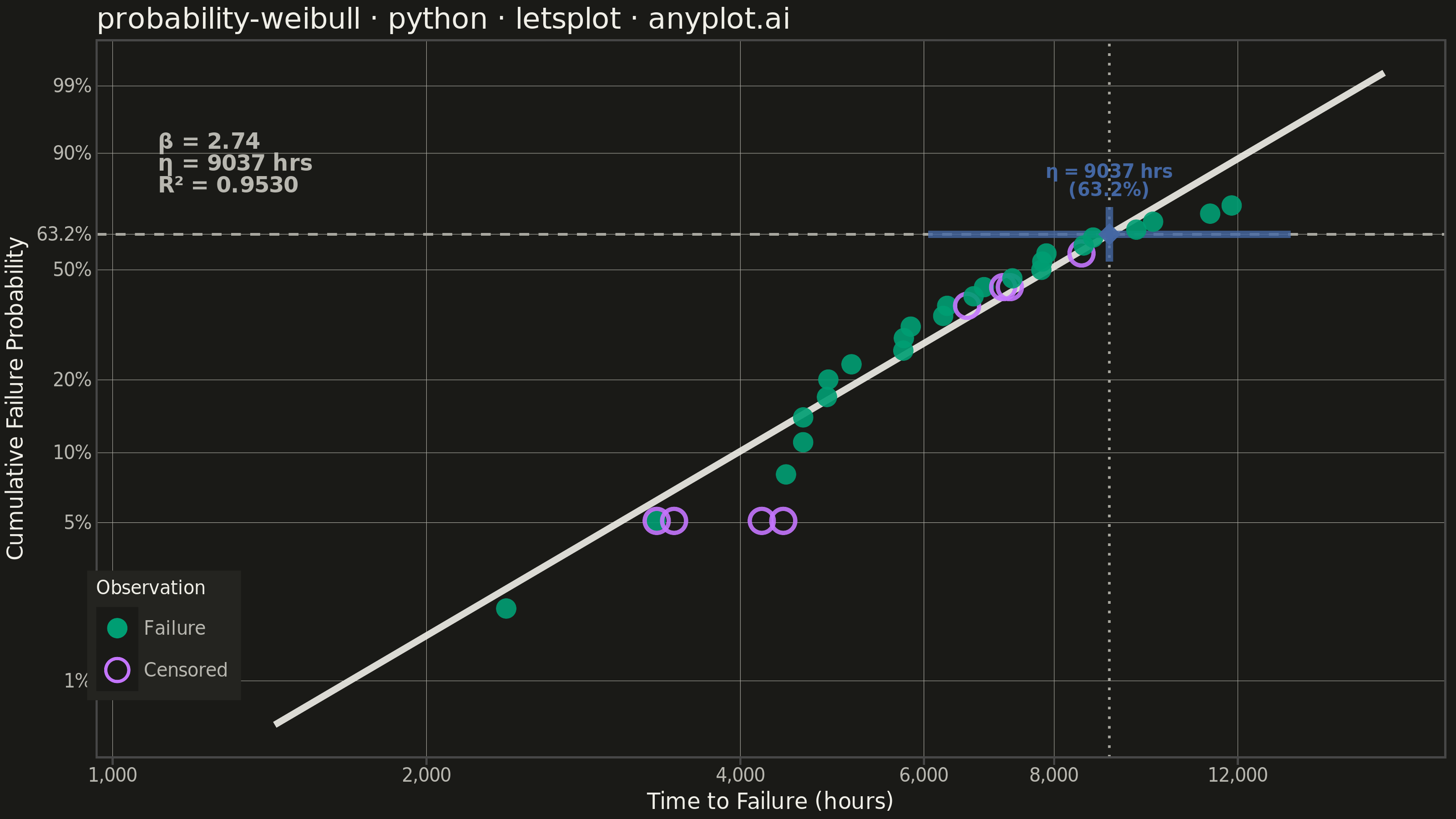
A Weibull probability plot displays failure or lifetime data on Weibull probability paper (logarithmic x-axis for time/cycles, linearized Weibull CDF on y-axis) with a fitted straight line. It is the standard tool in reliability engineering for estimating Weibull distribution parameters (shape and scale), assessing whether data follow a Weibull distribution, and extrapolating failure probabilities. The slope of the fitted line gives the shape parameter (beta), while the characteristic life (eta) is read at the 63.2% failure probability crossing.
""" anyplot.ai
probability-weibull: Weibull Probability Plot for Reliability Analysis
Library: letsplot 4.10.1 | Python 3.13.13
Quality: 86/100 | Updated: 2026-06-07
"""

# ruff: noqa: F403, F405, E402
"""anyplot.ai
probability-weibull: Weibull Probability Plot for Reliability Analysis
Library: letsplot | Python 3.13
Quality: pending | Created: 2026-06-07
"""

import os

import numpy as np
import pandas as pd
from lets_plot import *
from lets_plot.export import ggsave
from scipy import stats


LetsPlot.setup_html()

# Theme tokens (Imprint palette — see prompts/default-style-guide.md)
THEME = os.getenv("ANYPLOT_THEME", "light")
PAGE_BG = "#FAF8F1" if THEME == "light" else "#1A1A17"
ELEVATED_BG = "#FFFDF6" if THEME == "light" else "#242420"
INK = "#1A1A17" if THEME == "light" else "#F0EFE8"
INK_SOFT = "#4A4A44" if THEME == "light" else "#B8B7B0"
INK_MUTED = "#6B6A63" if THEME == "light" else "#A8A79F"

# Imprint palette — categorical (theme-independent)
BRAND = "#009E73"  # position 1 — Failure observations
COLOR_CENSORED = "#C475FD"  # position 2 — Censored observations
COLOR_ETA = "#4467A3"  # position 3 — characteristic life marker

# Data — Bearing wear-out fatigue: shape=3.2 (steep wear-out mode), scale=8000 h
np.random.seed(42)
shape_param = 3.2  # beta: wear-out failure mode (high shape → tight failure band)
scale_param = 8000  # eta: characteristic life in hours
n_failures = 25
n_censored = 8

failure_times = np.sort(stats.weibull_min.rvs(shape_param, scale=scale_param, size=n_failures))
censored_times = np.sort(np.random.uniform(3000, 10000, n_censored))

all_times = np.concatenate([failure_times, censored_times])
is_failure = np.concatenate([np.ones(n_failures), np.zeros(n_censored)])

sort_idx = np.argsort(all_times)
all_times = all_times[sort_idx]
is_failure = is_failure[sort_idx]

# Median rank plotting positions (Bernard's approximation): (i - 0.3) / (n + 0.4)
n_total = len(all_times)
failure_rank = np.cumsum(is_failure)
median_ranks = np.clip((failure_rank - 0.3) / (n_total + 0.4), 1e-6, 1 - 1e-6)

# Weibull linearization: y = ln(-ln(1 - F))
weibull_y = np.log(-np.log(1 - median_ranks))
log_times = np.log(all_times)

df_all = pd.DataFrame(
    {"log_time": log_times, "weibull_y": weibull_y, "status": np.where(is_failure == 1, "Failure", "Censored")}
)

df_failures = df_all[df_all["status"] == "Failure"].copy()

# Linear fit on Weibull-linearized failure points: beta = slope, eta = exp(-intercept/slope)
slope, intercept, r_value, _, _ = stats.linregress(df_failures["log_time"], df_failures["weibull_y"])
beta_fit = slope
eta_fit = np.exp(-intercept / slope)

# Fitted regression line spanning data range with padding
fit_x = np.linspace(np.log(all_times.min() * 0.6), np.log(all_times.max() * 1.4), 100)
fit_y = slope * fit_x + intercept
df_fit = pd.DataFrame({"log_time": fit_x, "weibull_y": fit_y})

# 63.2% characteristic life reference (where Weibull CDF = 1 - 1/e ≈ 0.632)
ref_y = np.log(-np.log(1 - 0.632))  # ≈ 0.0
log_eta = np.log(eta_fit)

# Y-axis ticks — Weibull probability scale
prob_levels = [0.01, 0.05, 0.10, 0.20, 0.50, 0.632, 0.90, 0.99]
y_ticks = [np.log(-np.log(1 - p)) for p in prob_levels]
y_labels = ["1%", "5%", "10%", "20%", "50%", "63.2%", "90%", "99%"]

# X-axis ticks — hours on log scale
x_vals = [1000, 2000, 4000, 6000, 8000, 12000]
x_ticks = [np.log(v) for v in x_vals]
x_labels = ["1,000", "2,000", "4,000", "6,000", "8,000", "12,000"]

# Crosshair segments emphasising the characteristic life intersection
df_h_seg = pd.DataFrame({"x": [log_eta - 0.4], "xend": [log_eta + 0.4], "y": [ref_y], "yend": [ref_y]})
df_v_seg = pd.DataFrame({"x": [log_eta], "xend": [log_eta], "y": [ref_y - 0.28], "yend": [ref_y + 0.28]})

# Characteristic life label — positioned above the crosshair to avoid data crowding
df_eta_label = pd.DataFrame({"x": [log_eta], "y": [ref_y + 0.55], "label": [f"η = {eta_fit:.0f} hrs\n(63.2%)"]})

# Parameter annotation — upper-left (high-probability region is sparse for wear-out data)
df_annot = pd.DataFrame(
    {
        "x": [x_ticks[0] + 0.1],
        "y": [y_ticks[-2] - 0.1],
        "label": [f"β = {beta_fit:.2f}\nη = {eta_fit:.0f} hrs\nR² = {r_value**2:.4f}"],
    }
)

TITLE = "probability-weibull · python · letsplot · anyplot.ai"

anyplot_theme = theme(
    plot_background=element_rect(fill=PAGE_BG, color=PAGE_BG),
    panel_background=element_rect(fill=PAGE_BG),
    panel_border=element_blank(),
    panel_grid_major=element_line(color=INK_MUTED, size=0.25),
    panel_grid_minor=element_blank(),
    axis_title=element_text(color=INK, size=12),
    axis_text=element_text(color=INK_SOFT, size=10),
    axis_line=element_line(color=INK_SOFT),
    plot_title=element_text(color=INK, size=16),
    legend_background=element_rect(fill=ELEVATED_BG, color=INK_SOFT),
    legend_text=element_text(color=INK_SOFT, size=10),
    legend_title=element_text(color=INK, size=10),
    legend_position=[0.05, 0.17],
)

# Plot
plot = (
    ggplot(df_all, aes(x="log_time", y="weibull_y", color="status", shape="status"))
    # Fitted regression line
    + geom_line(
        data=df_fit, mapping=aes(x="log_time", y="weibull_y"), color=INK, size=1.6, alpha=0.90, inherit_aes=False
    )
    # 63.2% horizontal reference
    + geom_hline(yintercept=ref_y, linetype="dashed", color=INK_MUTED, size=0.6)
    # Vertical reference at eta
    + geom_vline(xintercept=log_eta, linetype="dotted", color=INK_MUTED, size=0.6)
    # Crosshair emphasis at characteristic life intersection
    + geom_segment(
        data=df_h_seg,
        mapping=aes(x="x", y="y", xend="xend", yend="yend"),
        color=COLOR_ETA,
        size=1.8,
        alpha=0.8,
        inherit_aes=False,
    )
    + geom_segment(
        data=df_v_seg,
        mapping=aes(x="x", y="y", xend="xend", yend="yend"),
        color=COLOR_ETA,
        size=1.8,
        alpha=0.8,
        inherit_aes=False,
    )
    # Failure / censored data points (color + shape redundancy for accessibility)
    + geom_point(size=5, alpha=0.9, stroke=1.0)
    # Diamond marker at characteristic life intersection
    + geom_point(
        data=pd.DataFrame({"x": [log_eta], "y": [ref_y]}),
        mapping=aes(x="x", y="y"),
        color=COLOR_ETA,
        fill=COLOR_ETA,
        size=8,
        shape=18,
        alpha=0.95,
        inherit_aes=False,
    )
    # Characteristic life label above intersection to avoid crowding
    + geom_text(
        data=df_eta_label,
        mapping=aes(x="x", y="y", label="label"),
        size=5,
        color=COLOR_ETA,
        hjust=0.5,
        fontface="bold",
        inherit_aes=False,
    )
    # Weibull parameter annotation (upper-left, away from dense data region)
    + geom_text(
        data=df_annot,
        mapping=aes(x="x", y="y", label="label"),
        size=6,
        color=INK_SOFT,
        hjust=0,
        fontface="bold",
        inherit_aes=False,
    )
    + scale_color_manual(name="Observation", values={"Failure": BRAND, "Censored": COLOR_CENSORED})
    + scale_shape_manual(name="Observation", values={"Failure": 16, "Censored": 1})
    + scale_x_continuous(breaks=x_ticks, labels=x_labels)
    + scale_y_continuous(breaks=y_ticks, labels=y_labels)
    + labs(x="Time to Failure (hours)", y="Cumulative Failure Probability", title=TITLE)
    + ggsize(800, 450)
    + anyplot_theme
)

# Save
ggsave(plot, f"plot-{THEME}.png", path=".", scale=4)
ggsave(plot, f"plot-{THEME}.html", path=".")
Runnable source as JSON, for any HTTP client: https://api.anyplot.ai/specs/probability-weibull/letsplot/code. Any spec id and library id listed in llms-full.txt fit the same URL shape; every URL below is complete and callable.
{
  "spec_id": "probability-weibull",
  "language": "python",
  "library": "letsplot",
  "page": "https://anyplot.ai/probability-weibull/python/letsplot",
  "hub": "https://anyplot.ai/probability-weibull",
  "code_json": "https://api.anyplot.ai/specs/probability-weibull/letsplot/code",
  "spec_json": "https://api.anyplot.ai/specs/probability-weibull",
  "render_light_png": "https://storage.googleapis.com/anyplot-images/plots/probability-weibull/python/letsplot/plot-light.png",
  "render_dark_png": "https://storage.googleapis.com/anyplot-images/plots/probability-weibull/python/letsplot/plot-dark.png",
  "interactive_light_html": "https://storage.googleapis.com/anyplot-images/plots/probability-weibull/python/letsplot/plot-light.html",
  "interactive_dark_html": "https://storage.googleapis.com/anyplot-images/plots/probability-weibull/python/letsplot/plot-dark.html",
  "quality_score": 86.0,
  "license": "MIT",
  "guide": "https://anyplot.ai/llms.txt"
}
Part of Weibull Probability Plot for Reliability Analysis on anyplot.ai.