The same plot in 14 other libraries — Python: Altair, Bokeh, lets-plot, Matplotlib, Plotly, plotnine, Pygal, Seaborn; R: ggplot2; JavaScript: Chart.js, D3.js, Apache ECharts, Highcharts, MUI X Charts. Compare all 15 side by side: Weibull Probability Plot for Reliability Analysis in Python, R, Julia and JavaScript.
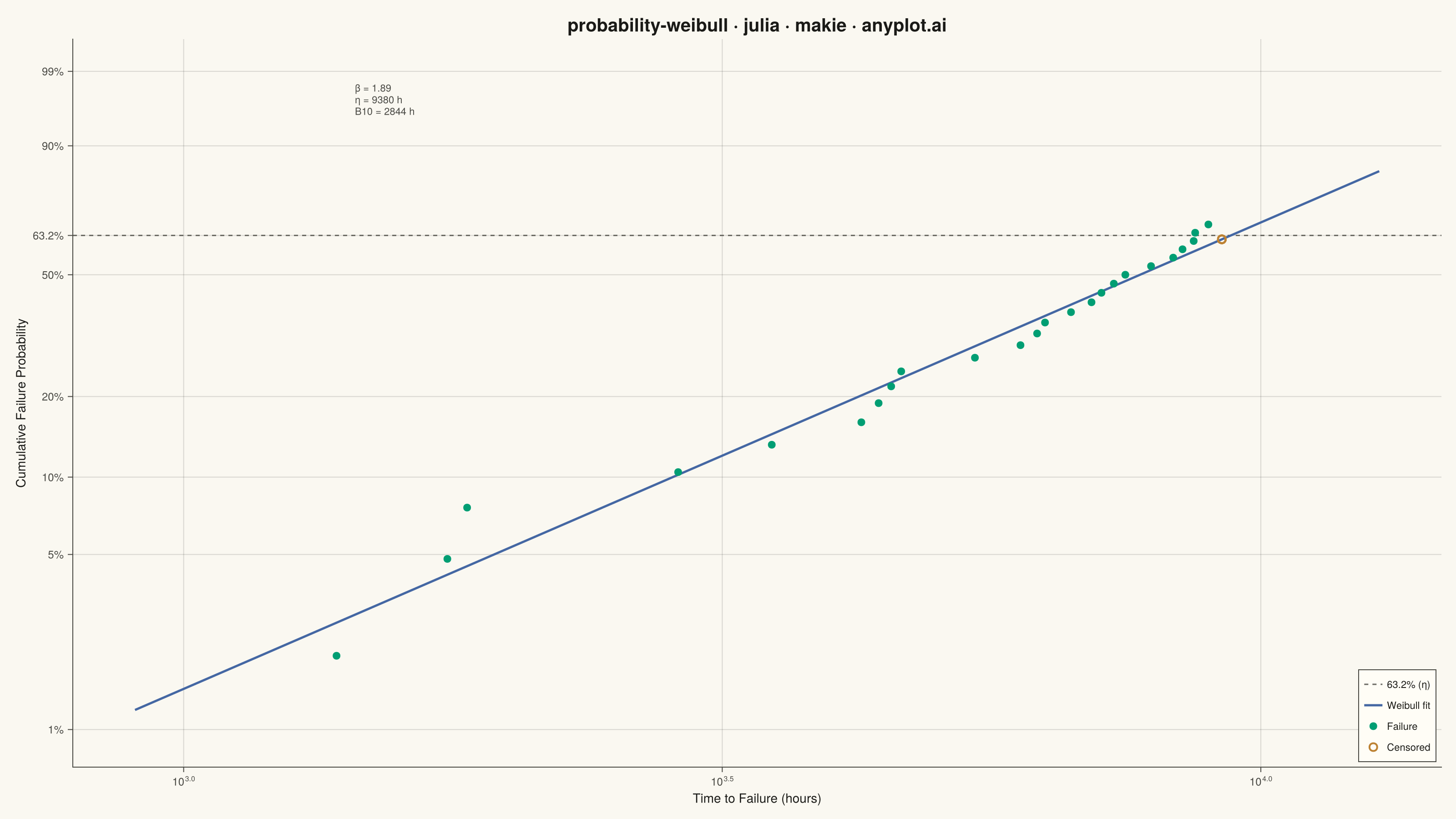
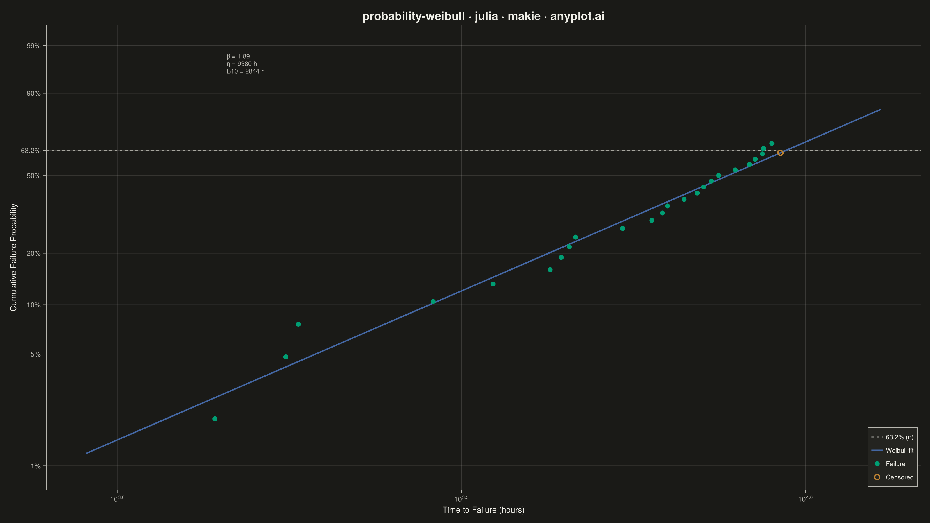
A Weibull probability plot displays failure or lifetime data on Weibull probability paper (logarithmic x-axis for time/cycles, linearized Weibull CDF on y-axis) with a fitted straight line. It is the standard tool in reliability engineering for estimating Weibull distribution parameters (shape and scale), assessing whether data follow a Weibull distribution, and extrapolating failure probabilities. The slope of the fitted line gives the shape parameter (beta), while the characteristic life (eta) is read at the 63.2% failure probability crossing.
# anyplot.ai
# probability-weibull: Weibull Probability Plot for Reliability Analysis
# Library: makie 0.22.10 | Julia 1.11.9
# Quality: 91/100 | Created: 2026-06-07

using CairoMakie
using Colors
using Random
using Statistics

Random.seed!(42)

# Theme tokens — Imprint palette
const THEME       = get(ENV, "ANYPLOT_THEME", "light")
const PAGE_BG     = THEME == "light" ? colorant"#FAF8F1" : colorant"#1A1A17"
const ELEVATED_BG = THEME == "light" ? colorant"#FFFDF6" : colorant"#242420"
const INK         = THEME == "light" ? colorant"#1A1A17" : colorant"#F0EFE8"
const INK_SOFT    = THEME == "light" ? colorant"#4A4A44" : colorant"#B8B7B0"
const INK_MUTED   = THEME == "light" ? colorant"#6B6A63" : colorant"#A8A79F"

const IMPRINT_PALETTE = [
    colorant"#009E73",  # 1 — brand green (failure data points)
    colorant"#C475FD",  # 2 — lavender
    colorant"#4467A3",  # 3 — blue (Weibull fit line)
    colorant"#BD8233",  # 4 — ochre (censored points)
    colorant"#AE3030",  # 5 — matte red
    colorant"#2ABCCD",  # 6 — cyan
    colorant"#954477",  # 7 — rose
    colorant"#99B314",  # 8 — lime
]

# Data: bearing fatigue-life qualification test (hours)
# True Weibull: shape β = 2.5, characteristic life η = 8500 h
n_total   = 35
beta_true = 2.5
eta_true  = 8500.0

all_lifetimes  = eta_true .* (-log.(rand(n_total))).^(1.0 / beta_true)
censor_time    = 9200.0   # inspection end time — survivors are right-censored here

observed_times  = min.(all_lifetimes, censor_time)
censored_mask   = all_lifetimes .> censor_time

# Sort all observations by observed time
order           = sortperm(observed_times)
times_sorted    = observed_times[order]
censored_sorted = censored_mask[order]

# Johnson's method: adjusted mean order number for each failure
# accounting for right-censored suspensions
adj_ranks, failure_times, cens_times = let
    prev = 0.0
    _ranks = Float64[]
    _ftimes = Float64[]
    _ctimes = Float64[]
    for i in 1:n_total
        if !censored_sorted[i]
            prev += (n_total + 1 - prev) / (n_total - i + 2)
            push!(_ranks, prev)
            push!(_ftimes, times_sorted[i])
        else
            push!(_ctimes, times_sorted[i])
        end
    end
    _ranks, _ftimes, _ctimes
end

# Bernard's median rank: F_i = (rank_i - 0.3) / (n + 0.4)
F_vals  = clamp.((adj_ranks .- 0.3) ./ (n_total + 0.4), 1e-6, 1.0 - 1e-6)

# Weibull linearization: y = ln(−ln(1−F)), x = ln(t)
log_t_fail = log.(failure_times)
y_fail     = log.(-log.(1.0 .- F_vals))

# OLS regression in linearized space → β̂, η̂
x_bar     = mean(log_t_fail)
y_bar     = mean(y_fail)
beta_hat  = sum((log_t_fail .- x_bar) .* (y_fail .- y_bar)) /
             sum((log_t_fail .- x_bar).^2)
intercept = y_bar - beta_hat * x_bar
eta_hat   = exp(-intercept / beta_hat)

# B10 life: time at which 10% of units have failed
t_b10 = exp((log(-log(1.0 - 0.10)) - intercept) / beta_hat)

# Fitted line spanning the observed time range
t_lo  = minimum(times_sorted) * 0.65
t_hi  = maximum(times_sorted) * 1.40
t_fit = exp.(range(log(t_lo), log(t_hi); length = 200))
y_fit = beta_hat .* log.(t_fit) .+ intercept

# Custom y-axis ticks on the Weibull probability scale
prob_pct    = [1.0, 5.0, 10.0, 20.0, 50.0, 63.2, 90.0, 99.0]
y_tick_vals = log.(-log.(1.0 .- prob_pct ./ 100.0))
y_tick_lbls = ["1%", "5%", "10%", "20%", "50%", "63.2%", "90%", "99%"]

# Grid color: INK at 15% opacity
grid_col = RGBAf(INK.r, INK.g, INK.b, 0.15f0)

# Figure
fig = Figure(
    size            = (1600, 900),
    fontsize        = 14,
    backgroundcolor = PAGE_BG,
)

ax = Axis(
    fig[1, 1];
    xscale            = log10,
    title             = "probability-weibull · julia · makie · anyplot.ai",
    titlesize         = 20,
    titlecolor        = INK,
    xlabel            = "Time to Failure (hours)",
    ylabel            = "Cumulative Failure Probability",
    xlabelsize        = 14,
    ylabelsize        = 14,
    xticklabelsize    = 12,
    yticklabelsize    = 12,
    xlabelcolor       = INK,
    ylabelcolor       = INK,
    xticklabelcolor   = INK_SOFT,
    yticklabelcolor   = INK_SOFT,
    xtickcolor        = INK_SOFT,
    ytickcolor        = INK_SOFT,
    backgroundcolor   = PAGE_BG,
    topspinevisible   = false,
    rightspinevisible = false,
    leftspinecolor    = INK_SOFT,
    bottomspinecolor  = INK_SOFT,
    xgridcolor        = grid_col,
    ygridcolor        = grid_col,
    yticks            = (y_tick_vals, y_tick_lbls),
)

# 63.2% reference line — time axis spans the full x range
y_632 = log(-log(1.0 - 0.632))
hlines!(ax, [y_632]; color = INK_MUTED, linewidth = 1.5, linestyle = :dash,
        label = "63.2% (η)")

# Fitted Weibull line
lines!(ax, t_fit, y_fit; color = IMPRINT_PALETTE[3], linewidth = 2.5,
       label = "Weibull fit")

# Failure observations — filled circles (first Imprint series, brand green)
scatter!(ax, failure_times, y_fail;
    color       = IMPRINT_PALETTE[1],
    markersize  = 12,
    marker      = :circle,
    strokewidth = 0,
    label       = "Failure",
)

# Censored observations — hollow circles at their time, y interpolated from fit
if length(cens_times) > 0
    y_cens = beta_hat .* log.(cens_times) .+ intercept
    scatter!(ax, cens_times, y_cens;
        color       = :transparent,
        strokecolor = IMPRINT_PALETTE[4],
        strokewidth = 2.0,
        markersize  = 12,
        marker      = :circle,
        label       = "Censored",
    )
end

# Parameter annotation (upper-left, away from dense data region)
ann_x   = t_lo * 1.6
ann_y   = y_tick_vals[end] - 0.10
ann_txt = "β = $(round(beta_hat, digits=2))\nη = $(round(Int, eta_hat)) h\nB10 = $(round(Int, t_b10)) h"
text!(ax, [ann_x], [ann_y];
    text    = [ann_txt],
    fontsize = 13,
    color   = INK_SOFT,
    align   = (:left, :top),
)

# B10 life graphical marker — vertical dashed line from bottom of plot to the 10% level
y_b10 = log(-log(1.0 - 0.10))
lines!(ax, [t_b10, t_b10], [y_tick_vals[1] - 0.35, y_b10];
    color     = INK_MUTED,
    linewidth = 1.5,
    linestyle = :dash,
)
scatter!(ax, [t_b10], [y_b10];
    color       = INK_SOFT,
    marker      = :diamond,
    markersize  = 10,
    strokewidth = 0,
)
text!(ax, [t_b10], [y_b10 + 0.08];
    text     = ["B10"],
    fontsize = 12,
    color    = INK_SOFT,
    align    = (:center, :bottom),
)

# Legend
axislegend(ax;
    position        = :rb,
    backgroundcolor = ELEVATED_BG,
    framecolor      = INK_SOFT,
    labelcolor      = INK,
    labelsize       = 11,
)

# Constrain y to the tick range with small padding
ylims!(ax, y_tick_vals[1] - 0.35, y_tick_vals[end] + 0.30)

save("plot-$(THEME).png", fig; px_per_unit = 2)
Runnable source as JSON, for any HTTP client: https://api.anyplot.ai/specs/probability-weibull/makie/code. Any spec id and library id listed in llms-full.txt fit the same URL shape; every URL below is complete and callable.
{
  "spec_id": "probability-weibull",
  "language": "julia",
  "library": "makie",
  "page": "https://anyplot.ai/probability-weibull/julia/makie",
  "hub": "https://anyplot.ai/probability-weibull",
  "code_json": "https://api.anyplot.ai/specs/probability-weibull/makie/code",
  "spec_json": "https://api.anyplot.ai/specs/probability-weibull",
  "render_light_png": "https://storage.googleapis.com/anyplot-images/plots/probability-weibull/julia/makie/plot-light.png",
  "render_dark_png": "https://storage.googleapis.com/anyplot-images/plots/probability-weibull/julia/makie/plot-dark.png",
  "quality_score": 91.0,
  "license": "MIT",
  "guide": "https://anyplot.ai/llms.txt"
}
Part of Weibull Probability Plot for Reliability Analysis on anyplot.ai.