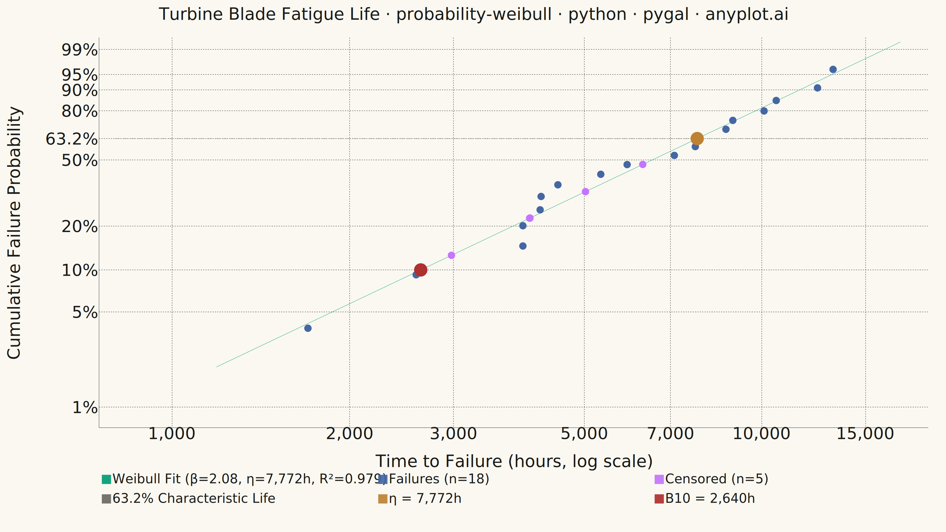
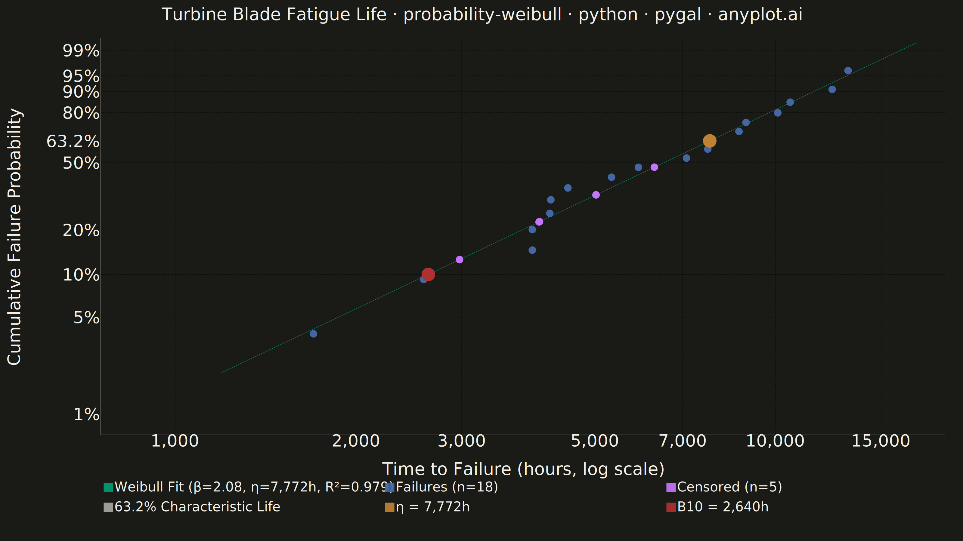
A Weibull probability plot displays failure or lifetime data on Weibull probability paper (logarithmic x-axis for time/cycles, linearized Weibull CDF on y-axis) with a fitted straight line. It is the standard tool in reliability engineering for estimating Weibull distribution parameters (shape and scale), assessing whether data follow a Weibull distribution, and extrapolating failure probabilities. The slope of the fitted line gives the shape parameter (beta), while the characteristic life (eta) is read at the 63.2% failure probability crossing.
""" anyplot.ai
probability-weibull: Weibull Probability Plot for Reliability Analysis
Library: pygal 3.1.0 | Python 3.13.13
Quality: 83/100 | Updated: 2026-06-07
"""

import os
import sys


# Remove the script's own directory so pygal.py doesn't shadow the installed pygal package
_here = os.path.dirname(os.path.abspath(__file__))
if _here in sys.path:
    sys.path.remove(_here)

import numpy as np
import pygal
from pygal.style import Style
from scipy import stats


# Theme tokens
THEME = os.getenv("ANYPLOT_THEME", "light")
PAGE_BG = "#FAF8F1" if THEME == "light" else "#1A1A17"
INK = "#1A1A17" if THEME == "light" else "#F0EFE8"
INK_SOFT = "#4A4A44" if THEME == "light" else "#B8B7B0"
INK_MUTED = "#6B6A63" if THEME == "light" else "#A8A79F"

# Imprint categorical palette — Weibull fit takes position 1 (brand green)
IMPRINT = ("#009E73", "#C475FD", "#4467A3", "#BD8233", "#AE3030", "#2ABCCD")

# Data — turbine blade fatigue-life (hours) with failures and suspensions
np.random.seed(42)
n_failures = 18
n_censored = 5
beta_true = 2.5
eta_true = 8000

failure_times = np.sort(stats.weibull_min.rvs(beta_true, scale=eta_true, size=n_failures))
censored_times = np.sort(np.random.uniform(2000, 9000, n_censored))

all_times = np.concatenate([failure_times, censored_times])
is_failure = np.concatenate([np.ones(n_failures), np.zeros(n_censored)])

sort_idx = np.argsort(all_times)
all_times = all_times[sort_idx]
is_failure = is_failure[sort_idx]

# Median rank plotting positions (i-0.3)/(n+0.4) for failures only
failure_ranks = np.cumsum(is_failure)
total_failures = failure_ranks[-1]
median_ranks = (failure_ranks - 0.3) / (total_failures + 0.4)

failure_mask = is_failure.astype(bool)
failure_x = all_times[failure_mask]
failure_prob = median_ranks[failure_mask]

# Weibull linearization: ln(-ln(1-F)) for y-axis, ln(time) for x-axis
weibull_y_failures = np.log(-np.log(1.0 - failure_prob))
ln_x_failures = np.log(failure_x)

# Fit line using least squares on linearized data
slope, intercept, r_value, _, _ = stats.linregress(ln_x_failures, weibull_y_failures)
beta_est = slope
eta_est = np.exp(-intercept / beta_est)

# Fitted line spanning full data range
x_fit_range = np.linspace(np.log(min(all_times) * 0.7), np.log(max(all_times) * 1.3), 100)
y_fit_line = slope * x_fit_range + intercept

# Censored points — placed on the fitted line at their log-time
censored_x = all_times[~failure_mask]
ln_censored_x = np.log(censored_x)
censored_y_on_line = slope * ln_censored_x + intercept

# 63.2% reference line (characteristic life)
ref_y = np.log(-np.log(1 - 0.632))

# B10 life: F=0.10 → time where 10% of units have failed
b10_y = np.log(-np.log(1 - 0.10))
b10_ln_x = (b10_y - intercept) / slope
b10_hours = np.exp(b10_ln_x)

# Characteristic life intersection on fitted line
eta_ln_x = (ref_y - intercept) / slope

# Axis tick values
x_tick_values = [1000, 2000, 3000, 5000, 7000, 10000, 15000]
x_tick_ln = [np.log(v) for v in x_tick_values]

prob_levels = [0.01, 0.05, 0.10, 0.20, 0.50, 0.632, 0.80, 0.90, 0.95, 0.99]
y_tick_weibull = [np.log(-np.log(1.0 - p)) for p in prob_levels]
y_tick_labels = [f"{p * 100:.1f}%" if p == 0.632 else f"{p * 100:.0f}%" for p in prob_levels]

# Axis bounds
x_min_ln = np.log(800)
x_max_ln = np.log(18000)
y_min_w = np.log(-np.log(1 - 0.008))
y_max_w = np.log(-np.log(1 - 0.993))

# Title fontsize scaled for title length (baseline 66 at 67 chars, floor 44)
title_str = "Turbine Blade Fatigue Life · probability-weibull · python · pygal · anyplot.ai"
title_font_size = max(44, round(66 * 67 / len(title_str)))

# Style — Imprint palette + theme-adaptive chrome
custom_style = Style(
    background=PAGE_BG,
    plot_background=PAGE_BG,
    foreground=INK,
    foreground_strong=INK,
    foreground_subtle=INK_MUTED,
    colors=(
        IMPRINT[0],  # fit line — brand green (Imprint pos 1)
        IMPRINT[2],  # failures — blue (Imprint pos 3)
        IMPRINT[1],  # censored — lavender (Imprint pos 2, lighter read than blue)
        INK_MUTED,  # 63.2% reference — theme-adaptive neutral
        IMPRINT[3],  # η marker — ochre (Imprint pos 4)
        IMPRINT[4],  # B10 marker — matte red (Imprint pos 5, reliability threshold)
    ),
    font_family="DejaVu Sans, Helvetica, Arial, sans-serif",
    title_font_family="DejaVu Sans, Helvetica, Arial, sans-serif",
    title_font_size=title_font_size,
    label_font_size=56,
    major_label_font_size=44,
    legend_font_size=44,
    legend_font_family="DejaVu Sans, Helvetica, Arial, sans-serif",
    value_font_size=36,
    tooltip_font_size=36,
    tooltip_font_family="DejaVu Sans, Helvetica, Arial, sans-serif",
    opacity=0.92,
    opacity_hover=1.0,
    stroke_opacity=1,
    stroke_opacity_hover=1,
)

# Chart configuration
chart = pygal.XY(
    width=3200,
    height=1800,
    style=custom_style,
    title=title_str,
    x_title="Time to Failure (hours, log scale)",
    y_title="Cumulative Failure Probability",
    show_legend=True,
    legend_at_bottom=True,
    legend_at_bottom_columns=3,
    legend_box_size=30,
    stroke=False,
    dots_size=10,
    show_x_guides=True,
    show_y_guides=True,
    margin_bottom=100,
    margin_left=90,
    margin_right=60,
    margin_top=60,
    truncate_legend=-1,
    range=(y_min_w, y_max_w),
    xrange=(x_min_ln, x_max_ln),
    print_values=False,
    print_zeroes=False,
    js=[],
    x_labels=[float(v) for v in x_tick_ln],
    y_labels=[float(v) for v in y_tick_weibull],
    x_value_formatter=lambda x: f"{np.exp(x):,.0f}h",
    value_formatter=lambda y: f"{(1 - np.exp(-np.exp(y))) * 100:.1f}%",
    tooltip_border_radius=10,
    tooltip_fancy_mode=True,
    dynamic_print_values=True,
)

# Override label display for axes
chart.y_labels = [{"value": float(v), "label": lbl} for v, lbl in zip(y_tick_weibull, y_tick_labels, strict=True)]
chart.x_labels = [{"value": float(v), "label": f"{int(t):,}"} for v, t in zip(x_tick_ln, x_tick_values, strict=True)]

# Fitted line — brand green (Imprint position 1)
fit_points = [(float(x), float(y)) for x, y in zip(x_fit_range, y_fit_line, strict=True)]
chart.add(
    f"Weibull Fit (β={beta_est:.2f}, η={eta_est:,.0f}h, R²={r_value**2:.3f})",
    fit_points,
    stroke=True,
    show_dots=False,
    stroke_style={"width": 8, "linecap": "round", "linejoin": "round"},
)

# Failure data points — blue (Imprint position 3)
failure_points = [
    {
        "value": (float(x), float(y)),
        "label": f"Failure at {np.exp(x):,.0f}h — F={((1 - np.exp(-np.exp(y))) * 100):.1f}%",
    }
    for x, y in zip(ln_x_failures, weibull_y_failures, strict=True)
]
chart.add(f"Failures (n={n_failures})", failure_points, stroke=False, dots_size=12)

# Censored data points — lavender (Imprint position 2), visually distinct from failures
censored_points = [
    {"value": (float(x), float(y)), "label": f"Censored at {np.exp(x):,.0f}h (suspended test)"}
    for x, y in zip(ln_censored_x, censored_y_on_line, strict=True)
]
chart.add(f"Censored (n={n_censored})", censored_points, stroke=False, dots_size=12)

# 63.2% reference line — theme-adaptive muted (structural reference, not data)
ref_line = [(float(x_min_ln), float(ref_y)), (float(x_max_ln), float(ref_y))]
chart.add(
    "63.2% Characteristic Life",
    ref_line,
    stroke=True,
    show_dots=False,
    stroke_style={"width": 6, "dasharray": "16, 10", "linecap": "round"},
)

# η marker — ochre (Imprint position 4), characteristic life
eta_marker = [
    {"value": (float(eta_ln_x), float(ref_y)), "label": f"η = {eta_est:,.0f}h (Characteristic Life at 63.2%)"}
]
chart.add(
    f"η = {eta_est:,.0f}h",
    eta_marker,
    stroke=False,
    dots_size=22,
    print_values=True,
    formatter=lambda x: f"η = {eta_est:,.0f}h",
)

# B10 marker — matte red (Imprint position 5), 10% reliability threshold
b10_marker = [{"value": (float(b10_ln_x), float(b10_y)), "label": f"B10 = {b10_hours:,.0f}h (10% Failure Life)"}]
chart.add(
    f"B10 = {b10_hours:,.0f}h",
    b10_marker,
    stroke=False,
    dots_size=22,
    print_values=True,
    formatter=lambda x: f"B10 = {b10_hours:,.0f}h",
)

# Save
chart.render_to_png(f"plot-{THEME}.png")
chart.render_to_file(f"plot-{THEME}.html")
Runnable source as JSON, for any HTTP client: https://api.anyplot.ai/specs/probability-weibull/pygal/code. Any spec id and library id listed in llms-full.txt fit the same URL shape; every URL below is complete and callable.
{
  "spec_id": "probability-weibull",
  "language": "python",
  "library": "pygal",
  "page": "https://anyplot.ai/probability-weibull/python/pygal",
  "hub": "https://anyplot.ai/probability-weibull",
  "code_json": "https://api.anyplot.ai/specs/probability-weibull/pygal/code",
  "spec_json": "https://api.anyplot.ai/specs/probability-weibull",
  "render_light_png": "https://storage.googleapis.com/anyplot-images/plots/probability-weibull/python/pygal/plot-light.png",
  "render_dark_png": "https://storage.googleapis.com/anyplot-images/plots/probability-weibull/python/pygal/plot-dark.png",
  "interactive_light_html": "https://storage.googleapis.com/anyplot-images/plots/probability-weibull/python/pygal/plot-light.html",
  "interactive_dark_html": "https://storage.googleapis.com/anyplot-images/plots/probability-weibull/python/pygal/plot-dark.html",
  "quality_score": 83.0,
  "license": "MIT",
  "guide": "https://anyplot.ai/llms.txt"
}
Part of Weibull Probability Plot for Reliability Analysis on anyplot.ai.