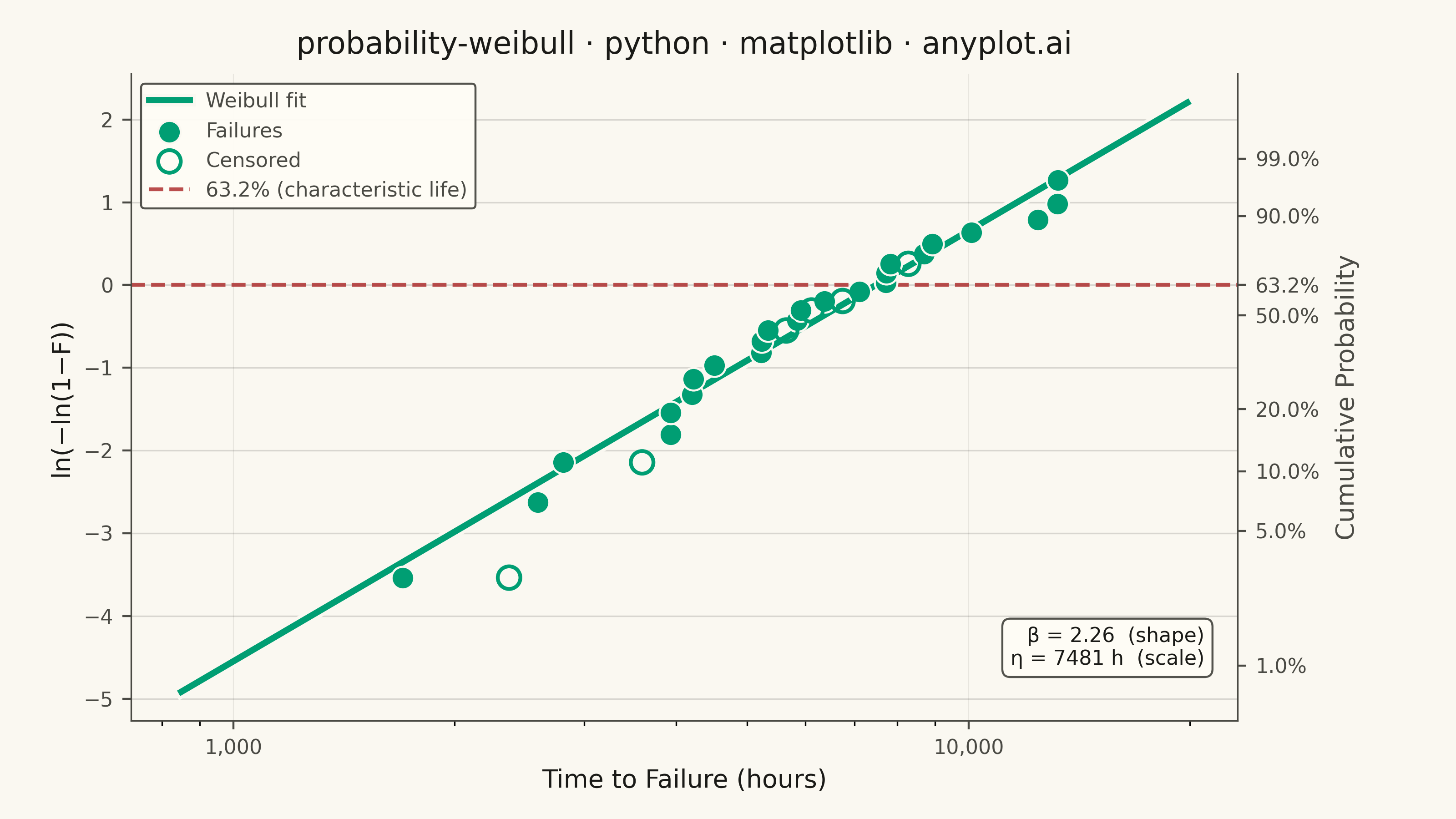
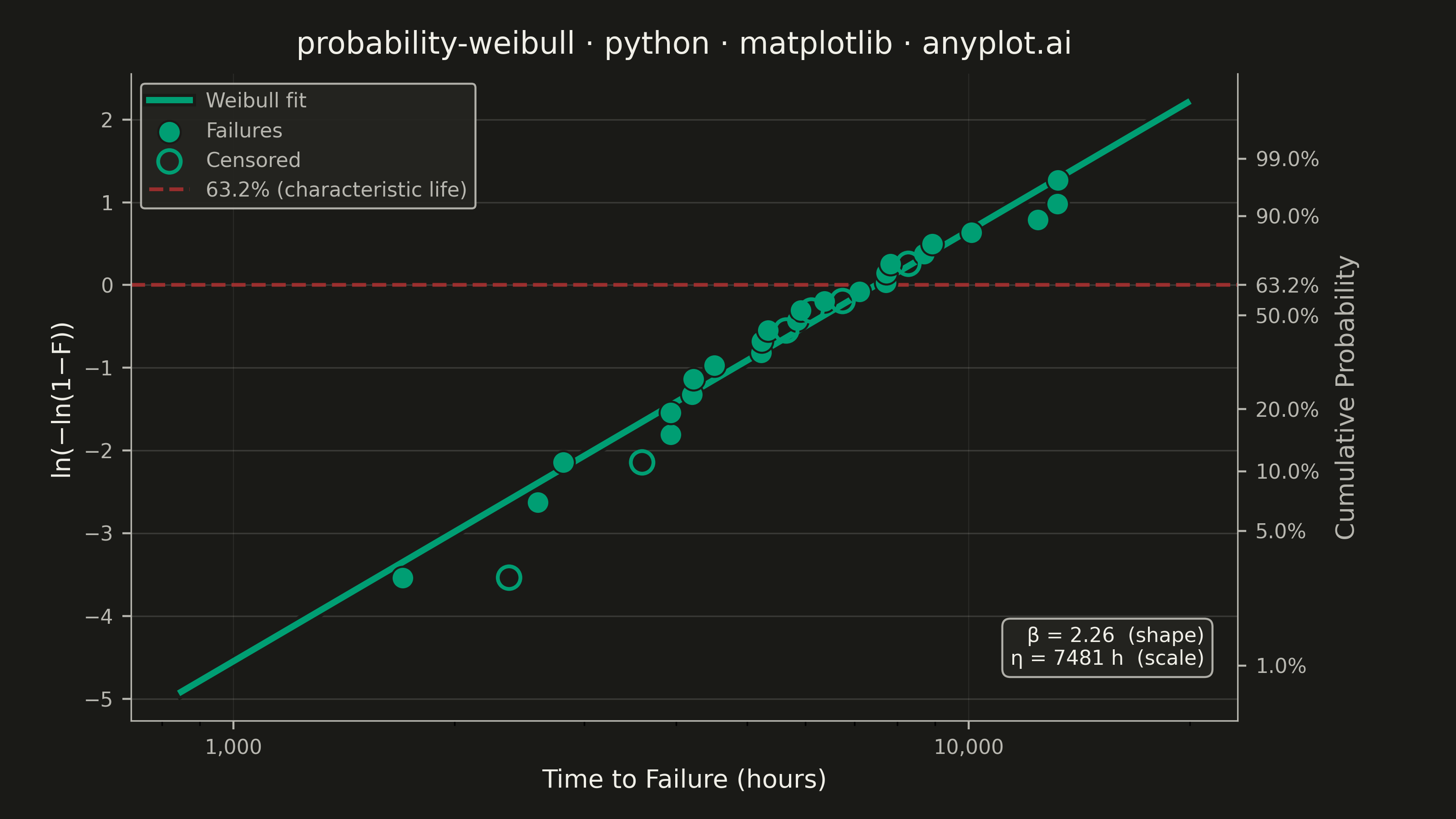
A Weibull probability plot displays failure or lifetime data on Weibull probability paper (logarithmic x-axis for time/cycles, linearized Weibull CDF on y-axis) with a fitted straight line. It is the standard tool in reliability engineering for estimating Weibull distribution parameters (shape and scale), assessing whether data follow a Weibull distribution, and extrapolating failure probabilities. The slope of the fitted line gives the shape parameter (beta), while the characteristic life (eta) is read at the 63.2% failure probability crossing.
""" anyplot.ai
probability-weibull: Weibull Probability Plot for Reliability Analysis
Library: matplotlib 3.10.9 | Python 3.13.13
Quality: 90/100 | Updated: 2026-06-07
"""

import os
import sys


# Remove the script's own directory from sys.path so 'import matplotlib' resolves
# to the installed package rather than this file (naming-conflict guard).
_script_dir = os.path.dirname(os.path.abspath(__file__))
sys.path = [p for p in sys.path if os.path.abspath(p or ".") != _script_dir]

import matplotlib.pyplot as plt
import matplotlib.ticker as ticker
import numpy as np
from matplotlib.patheffects import withStroke
from scipy import stats


# Theme-adaptive chrome — Imprint palette
THEME = os.getenv("ANYPLOT_THEME", "light")
PAGE_BG = "#FAF8F1" if THEME == "light" else "#1A1A17"
ELEVATED_BG = "#FFFDF6" if THEME == "light" else "#242420"
INK = "#1A1A17" if THEME == "light" else "#F0EFE8"
INK_SOFT = "#4A4A44" if THEME == "light" else "#B8B7B0"
INK_MUTED = "#6B6A63" if THEME == "light" else "#A8A79F"

# Imprint palette — first series brand green; semantic red for threshold line
IMPRINT_PALETTE = ["#009E73", "#C475FD", "#4467A3", "#BD8233", "#AE3030", "#2ABCCD", "#954477", "#99B314"]
BRAND = IMPRINT_PALETTE[0]  # "#009E73" — failures + fit (first categorical series)
RED = IMPRINT_PALETTE[4]  # "#AE3030" — 63.2% reference (semantic alarm threshold)

# Data — turbine blade fatigue-life (hours)
np.random.seed(42)
shape_true, scale_true = 2.5, 8000
n_total = 30
n_failures = 24
n_censored = n_total - n_failures

failure_times = np.sort(stats.weibull_min.rvs(shape_true, scale=scale_true, size=n_failures))
failure_times[2] *= 0.75  # early outlier — adds diagnostic interest
failure_times[-3] *= 1.25  # late outlier
censored_times = np.sort(np.random.uniform(2000, 10000, size=n_censored))

all_times = np.concatenate([failure_times, censored_times])
is_censored = np.concatenate([np.zeros(n_failures, dtype=bool), np.ones(n_censored, dtype=bool)])
sort_idx = np.argsort(all_times)
all_times = all_times[sort_idx]
is_censored = is_censored[sort_idx]

# Median rank plotting positions (Benard's approximation)
failure_indices = np.where(~is_censored)[0]
failure_times_sorted = all_times[failure_indices]
ranks = np.arange(1, len(failure_times_sorted) + 1)
median_rank = (ranks - 0.3) / (len(failure_times_sorted) + 0.4)

# Weibull linearized transform: ln(-ln(1-F))
weibull_y = np.log(-np.log(1 - median_rank))

# Least-squares fit on log(time) vs Weibull_y
log_times = np.log(failure_times_sorted)
slope, intercept = np.polyfit(log_times, weibull_y, 1)
beta = slope
eta = np.exp(-intercept / beta)

# Censored plotting positions (interpolated from adjacent median ranks)
censored_indices = np.where(is_censored)[0]
censored_times_vals = all_times[censored_indices]
censored_y_positions = []
for ct in censored_times_vals:
    idx = np.searchsorted(failure_times_sorted, ct, side="right")
    if idx == 0:
        f_val = 0.05
    elif idx >= len(median_rank):
        f_val = median_rank[-1]
    else:
        f_val = median_rank[idx - 1]
    censored_y_positions.append(np.log(-np.log(1 - min(f_val, 0.99))))
censored_y_positions = np.array(censored_y_positions)

# Fit line coordinates
fit_x = np.linspace(np.min(failure_times_sorted) * 0.5, np.max(failure_times_sorted) * 1.5, 200)
fit_y = beta * np.log(fit_x) - beta * np.log(eta)

# 63.2% reference — characteristic life (where Weibull CDF = 1 - 1/e)
y_632 = np.log(-np.log(1 - 0.632))

# Explicit y range for reliable twinx sync
all_y = np.concatenate([weibull_y, censored_y_positions, fit_y])
y_pad = 0.35
y_min = float(all_y.min()) - y_pad
y_max = float(all_y.max()) + y_pad

# Canvas — 3200×1800 px (landscape 16:9)
fig, ax = plt.subplots(figsize=(8, 4.5), dpi=400, facecolor=PAGE_BG)
ax.set_facecolor(PAGE_BG)

# Fit line with PathEffects halo — separates it visually from dense marker clusters
ax.plot(
    fit_x,
    fit_y,
    color=BRAND,
    linewidth=2.5,
    zorder=2,
    label="Weibull fit",
    path_effects=[withStroke(linewidth=5, foreground=PAGE_BG)],
)

# Failure markers (filled)
ax.scatter(
    failure_times_sorted, weibull_y, s=80, color=BRAND, edgecolors=PAGE_BG, linewidth=0.8, zorder=3, label="Failures"
)

# Censored markers (hollow — visually distinct from failures per spec)
ax.scatter(
    censored_times_vals,
    censored_y_positions,
    s=80,
    facecolors="none",
    edgecolors=BRAND,
    linewidth=1.5,
    zorder=3,
    label="Censored",
)

# 63.2% reference line (semantic red = alarm / design threshold)
ax.axhline(y=y_632, color=RED, linewidth=1.5, linestyle="--", alpha=0.85, zorder=1, label="63.2% (characteristic life)")

# Weibull parameter annotation
ax.text(
    0.97,
    0.08,
    f"β = {beta:.2f}  (shape)\nη = {eta:.0f} h  (scale)",
    transform=ax.transAxes,
    fontsize=8,
    ha="right",
    va="bottom",
    color=INK,
    bbox={
        "boxstyle": "round,pad=0.4",
        "facecolor": ELEVATED_BG,
        "edgecolor": INK_SOFT,
        "alpha": 0.95,
        "linewidth": 0.8,
    },
)

# Set primary y-axis limits before twinx
ax.set_ylim(y_min, y_max)

# Secondary y-axis — cumulative probability labels (bridges raw Weibull scale)
prob_levels = [0.01, 0.05, 0.10, 0.20, 0.50, 0.632, 0.90, 0.99]
prob_y_ticks = [np.log(-np.log(1 - p)) for p in prob_levels]
ax2 = ax.twinx()
ax2.set_ylim(y_min, y_max)
ax2.set_yticks(prob_y_ticks)
ax2.set_yticklabels([f"{p * 100:.1f}%" for p in prob_levels])
ax2.tick_params(axis="y", labelsize=8, colors=INK_SOFT, labelcolor=INK_SOFT)
ax2.spines["top"].set_visible(False)
ax2.spines["left"].set_visible(False)
ax2.spines["bottom"].set_visible(False)
ax2.spines["right"].set_color(INK_SOFT)
ax2.spines["right"].set_linewidth(0.6)
ax2.set_ylabel("Cumulative Probability", fontsize=10, color=INK_SOFT, labelpad=6)

# Title — length-adapted fontsize to avoid overflow
title = "probability-weibull · python · matplotlib · anyplot.ai"
title_fontsize = max(8, round(12 * 67 / len(title))) if len(title) > 67 else 12
ax.set_title(title, fontsize=title_fontsize, fontweight="medium", color=INK, pad=8)

# Primary axes labels and ticks
ax.set_xscale("log")
ax.set_xlabel("Time to Failure (hours)", fontsize=10, color=INK, labelpad=4)
ax.set_ylabel("ln(−ln(1−F))", fontsize=10, color=INK, labelpad=4)
ax.tick_params(axis="both", labelsize=8, colors=INK_SOFT, labelcolor=INK_SOFT)
ax.xaxis.set_major_formatter(ticker.FuncFormatter(lambda x, _: f"{x:,.0f}"))

# Spines — L-shaped frame
ax.spines["top"].set_visible(False)
ax.spines["right"].set_visible(False)
for spine in ("bottom", "left"):
    ax.spines[spine].set_color(INK_SOFT)
    ax.spines[spine].set_linewidth(0.6)

# Grid — subtle, y-axis heavier than x
ax.yaxis.grid(True, alpha=0.15, linewidth=0.6, color=INK)
ax.xaxis.grid(True, alpha=0.08, linewidth=0.4, color=INK)
ax.set_axisbelow(True)

# Legend
leg = ax.legend(fontsize=8, loc="upper left", framealpha=0.95)
if leg:
    leg.get_frame().set_facecolor(ELEVATED_BG)
    leg.get_frame().set_edgecolor(INK_SOFT)
    leg.get_frame().set_linewidth(0.8)
    plt.setp(leg.get_texts(), color=INK_SOFT)

# Margins — leave room for right y-axis label; no bbox_inches='tight' on savefig
fig.subplots_adjust(left=0.09, right=0.85, top=0.91, bottom=0.12)
plt.savefig(f"plot-{THEME}.png", dpi=400, facecolor=PAGE_BG)
Runnable source as JSON, for any HTTP client: https://api.anyplot.ai/specs/probability-weibull/matplotlib/code. Any spec id and library id listed in llms-full.txt fit the same URL shape; every URL below is complete and callable.
{
  "spec_id": "probability-weibull",
  "language": "python",
  "library": "matplotlib",
  "page": "https://anyplot.ai/probability-weibull/python/matplotlib",
  "hub": "https://anyplot.ai/probability-weibull",
  "code_json": "https://api.anyplot.ai/specs/probability-weibull/matplotlib/code",
  "spec_json": "https://api.anyplot.ai/specs/probability-weibull",
  "render_light_png": "https://storage.googleapis.com/anyplot-images/plots/probability-weibull/python/matplotlib/plot-light.png",
  "render_dark_png": "https://storage.googleapis.com/anyplot-images/plots/probability-weibull/python/matplotlib/plot-dark.png",
  "quality_score": 90.0,
  "license": "MIT",
  "guide": "https://anyplot.ai/llms.txt"
}
Part of Weibull Probability Plot for Reliability Analysis on anyplot.ai.